Week-4 Challenge WOT Condition Part-2

1. What is the difference between mapped and dynamic model of engine, motor and generator? How can you change model type? 
2. How does the model calculate miles per gallon? Which factors are considered to model fuel flow? 
3. Run the HEV ReferenceApplication with WOT drive cycle. Change the grade and wind velocity in the environment block. Comment on the results.
4. Keeping all other parameters same, compare the simulated results of hybrid and pure electric powertrains. 

m: To study and perform the following condition by using Powertrain Blockset.

Objective:

1. To study the difference between mapped and dynamic model of engine, motor and generator.and also How can we change model type? 
2. To describe how does the model calculate miles per gallon? and Which factors are considered to model fuel flow? 
3. To run the HEV ReferenceApplication with WOT drive cycle. Change the grade and wind velocity in the environment block. Comment on the results.
4. To compare the simulated results of hybrid and pure electric powertrains by keeping all other parameters same.  

Powertrain Blockset:

Powertrain Blockset provides fully assembled reference application models of automotive powertrains, including gasoline, diesel, hybrid, and electric systems. It includes a component library for simulating engine subsystems, transmission assemblies, traction motors, battery packs, and controller models. Powertrain Blockset also includes a dynamometer model for virtual testing. MDF file support provides a standards-based interface to calibration tools for data import.

Powertrain Blockset provides a standard model architecture that can be reused throughout the development process. We can use it for design tradeoff analysis and component sizing, control parameter optimization, and hardware-in-the-loop testing. We can customize models by parameterizing components in a reference application with our own data or by replacing a subsystem with our own model.

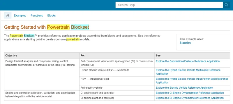
Powertrain Blockset provides a set of fully assembled reference applications, including gasoline (spark-ignition, SI), diesel (compression-ignition, CI), hybrid, and electric vehicle systems, as a starting point for our powertrain system model. To model a powertrain system for our project, we can select a reference application based on the powertrain type. Each reference application includes plant models, controllers, a longitudinal driver, and drive cycle data.

The reference applications come with a Simulink Projects configuration. Simulink Projects enables management and version control for top-level model files, component model files, and scripts.

Reference applications serve as a starting point for our system model. To tailor a reference application to our powertrain project, parameterize the components in the reference application using data from a domain-specific tool, a test bench, or a vehicle. Depending on our application and powertrain configuration, we might need to select the type of component models and further customize the system model.

The component library in Powertrain Blockset provides blocks of physical systems and controllers for:

• Propulsion
• Transmission
• Drivetrain
• Energy storage
• Longitudinal vehicle dynamics
• Drive cycle data and longitudinal driver

All the models in Powertrain Blockset, including the reference applications and components in the library, are fully open for customization. You can use Simulink Projects to manage model variants including variant selection, version management, and comparison.

Q1. a) What is the difference between mapped and dynamic model of engine, motor and generator?

Powertrain Blockset provides two types of combustion engine models: mapped and dynamic. 

Maped Model: Mapped Models represent the macro behaviour of the subsystem as a set of lookup tables. These models are useful for understanding the behaviour of the system using empirical data.

Dynamic Models: A dynamic model performs a real-time simulation of components that actually takes place in an original system to generate an output, depending upon random input situations. Dynamic models are suitable for designing control, estimator, and diagnostic algorithms that depend on dynamic subsystem states, like in closed-loop AFR control algorithm development.

Maped Model Engine: Mapped model of an engine represent macro engine behavior as a set of lookup tables (brake torque, fuel flow, air mass flow, exhaust temperature, efficiency, and emissions) as functions of commanded load and measured engine speed.

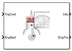
                    Mapped SI Engine

Dynamic Model Engine: Dynamic Model of an Engine performs a real-time simulation of components that actually takes place in an original system to generate an output and also the dynamic model of an engine decomposes engine behavior into individual component models that account for engine dynamics, most notably intake airflow and turbocharger dynamics. 

 

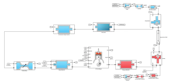
                                            Dynamic Model Engine

 Mapped Model Motor: The behaviour of the macro motor can be represented as a set of lookup tables of efficiency, torque curve, rpm, power curve, Temp. etc. 

 

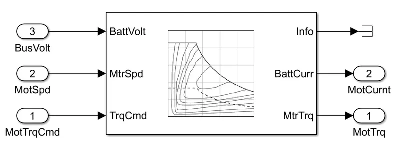
                                                       Mapped Model Motor

 

Dynamic Model Motor:  Dynamic Model of a motor performs a real-time simulation of components that actually takes place in an original system to generate an output and also the dynamic model of a motor decomposes motor behavior into individual component models.

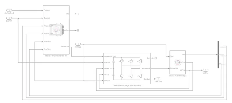
                                                         Dynamic Model Motor 

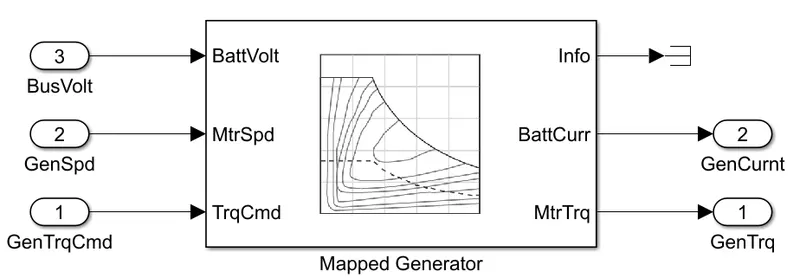
 Mapped Model Generator: The behavoiur of the Macro generator can be represented as a set of lookup tables of generator efficiency, motor torque, etc.

 

Dynamic Model Generator: Dynamic Model of a generator performs a real-time simulation of components that actually takes place in an original system to generate an output and also the dynamic model of a generator decomposes generator behavior into individual component models.

 

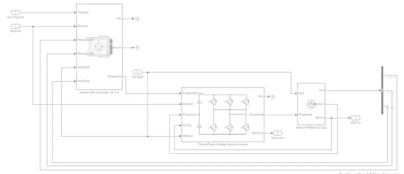
                                                              Dynamic Model Motor

 Q1. b) How can we change the model Type?

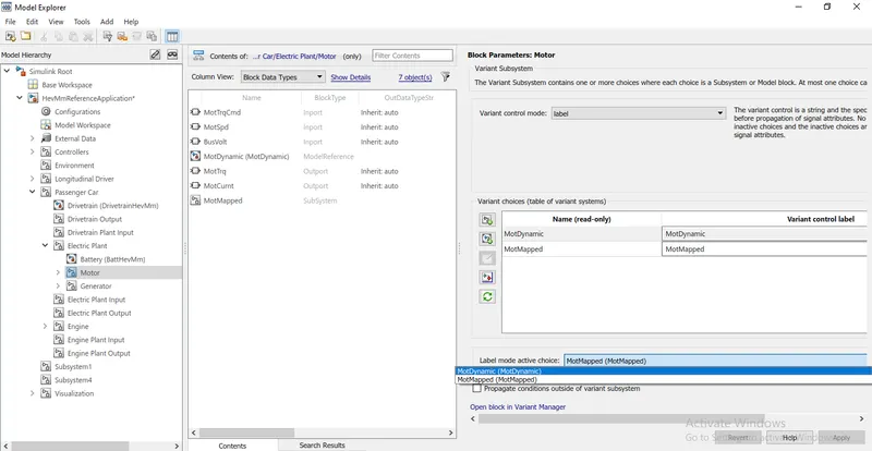
We can change the model type from mapped to dynamic and from dynamic to mapped based on the application.

• At first, we have to open the powertrain blockset module in Matlab documentation for the required vehicle.
• Then we have to click on passenger car or vehicle block and have to select the electric plant.
• Next, we have to Right-click on Engine/motor/generator on the vehicle model and have to select subsystem & model reference.
• In subsystem & model reference we have to select the option convert to the variant subsystem.

 The above process is given below,

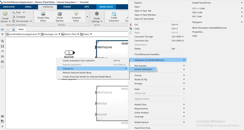
• Then by using model explorer we can change the model type. The following process is shown below,

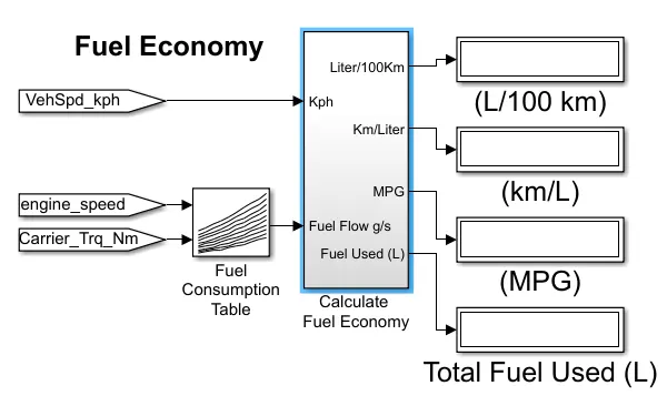
Q2. a)How does the model calculate miles per gallon?

 Miles Per Gallon: Miles per gallon(mpg) are commonly used in the United States, the United Kingdom, and Canada (alongside L/100 km). Kilometers per liter (km/L) are more commonly used elsewhere in the Americas, Asia, parts of Africa, and Oceania. When the mpg unit is used, it is necessary to identify the type of gallon used: the imperial gallon is 4.54609 liters, and the U.S. gallon is 3.785 liters. When using a measure expressed as distance per fuel unit, a higher number means more efficient, while a lower number means less efficient.

The Power train block set in Matlab has a model that calculates the miles per gallon for all kinds of vehicles.

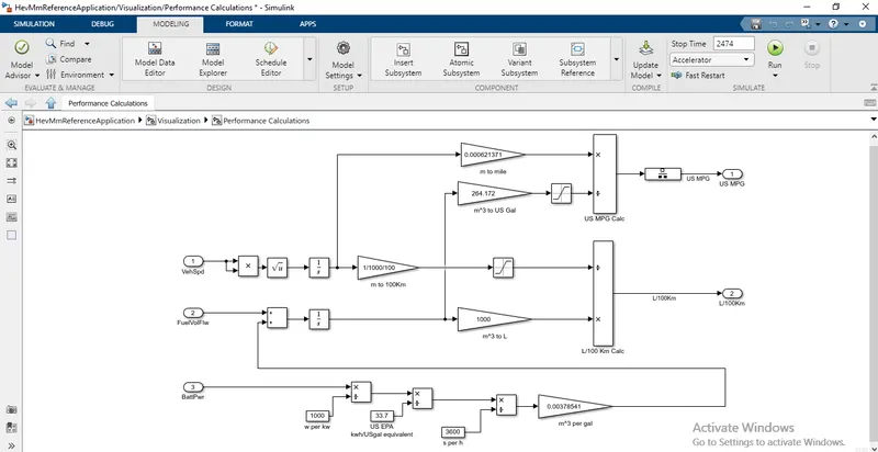
 The above model is for HEV which takes the input of the vehicle speed, Fuel Flow, and Battery power to calculate the fuel consumption and the equivalent battery consumption and calculates the miles per gallon.

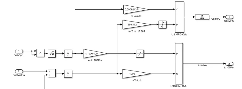
Vehicle Speed and Fuel Flow:

• To determine the fuel consumption throughout the drive cycle the vehicle speed is an important factor while considering the fuel consumption at that particular time.
• To convert speed to Distance we can integrate speed with time and also we are doing the same of converting the velocity to get the distance covered by integrating. 
• Then the fuel flow is expressed as the mass flow rate i.e the amount of fuel at each moment in kg/Sec. Now integrating this will result in the mass of the fuel and by dividing the mass with the fuel density we can convert it to the volume and by multiplying 1000 we can get it in liters.
• By comparing the results we can get the amount of the consumed to Run for 100 km. 

The Vehicle Speed and Fuel Flow model is given below.

Battery Power:

• The amount of energy of battery power equivalent to that of the Engine is calculated here.
• Then the battery power is converted to kW by dividing it by 1000.
• Battery power is then converted into energy kWh by multiplying it with time.
• Then converting the Energy from kWh to equivalent energy in US gallons of automotive gasoline by dividing with 33.7. Since we get the energy in US Gallons equal in kWh, to get the energy of equivalent US Gallons per second we have to divide with 3600 and have to convert the hour to seconds. 
• Then US Gallon per second is multiplied by 0.00378541 to get the volume of fuel flow in `m^3`/s.And also it is multiplied with 739(density of gasoline) to get the mass flow rate in kg/s.
• Then finally the Battery energy equivalent in kg/s is given as an input for the fuel flow to find the equivalent US gallons of energy and estimate the Miles per Gallon. 

The Battery Power model is given below.

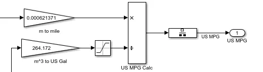
Calculating Miles per Gallon:

• The inputs from the vehicle speed i.e the distance we found (in meters) are taken into the calculation and it is converted to the miles by multiplying with 0.000621371.
• Then the inputs from fuel flow (Battery energy + Fuel energy) which is in `m^3` are converted into equivalent US Gallons by multiplying with 264.172.
• Then the two inputs Miles covered and equivalent US Gallon are further divided and the final result is got in Miles/Gallon.

Q2. b)Which factors are considered to model fuel flow?

Factors considered in the model fuel flow are Fuel Economy and Fuel Consumption.

• Fuel Economy: The fuel economy of an automobile relates to distance by a vehicle and the amount of fuel consumed. Consumption can be expressed in terms of the volume of fuel to travel a distance, or the distance traveled per unit volume of fuel consumed. Different methods are used to approximate the actual performance of the vehicle.The energy in the fuel is required to overcome various losses (like wind resistance, tire drag, and others parameters) encountered while propelling the vehicle, and in providing power to vehicle systems such as ignition or air conditioning. Driver's behavior can affect fuel economy such as sudden acceleration and heavy braking waste energy.

The Major factors that are considered in the Fuel Economy :

1. Vehicle Speed
2. Engine Speed
3. Motor Torque

• Fuel Consumption: Fuel Consumption is the inverse of fuel economy. It is the amount of fuel consumed in driving with a given distance.

Q3.Run the HEV ReferenceApplication with WOT drive cycle. Change the grade and wind velocity in the environment block. Comment on the results.

 Hybrid Electric Vehicle: A hybrid electric vehicle (HEV) is a type of hybrid vehicle that combines a conventional internal combustion engine(ICE) system with an electric propulsion system (hybrid vehicle drivetrain). The presence of the electric powertrain is intended to achieve either better fuel economy than a conventional vehicle or better performance. There is a variety of HEV types and the degree to which each function as an electric vehicle (EV) also varies. The most common form of HEV is the hybrid electric car, although hybrid electric trucks (pickups and tractors), buses, boats and aircraft also exist. An example of a Hybrid Electric Vehicle is Toyota Prius which is the world's best-selling Hybrid Car.

 

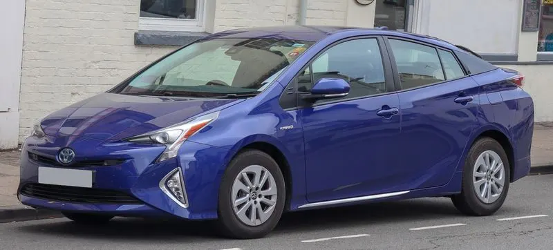
                                                                    Toyota Prius

 

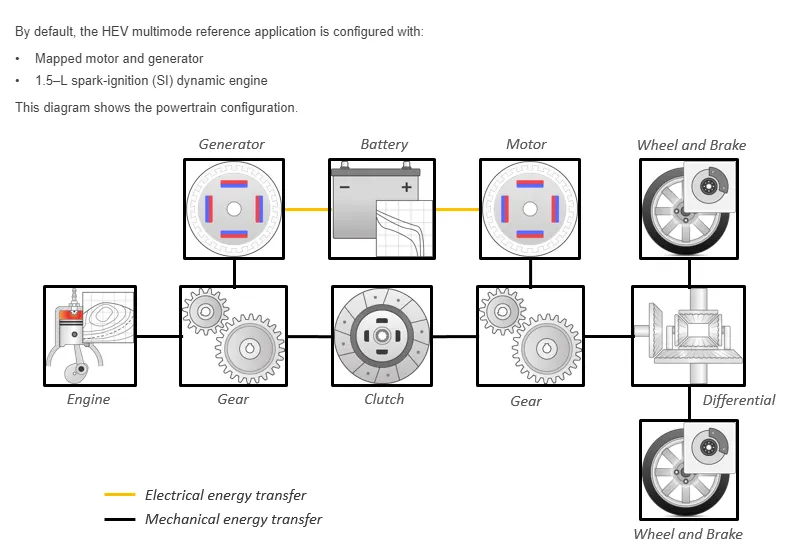
Architecture: 

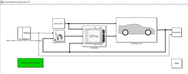
Simulation Model: 

 

 Case 1:

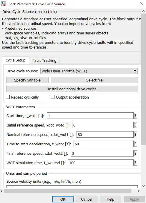
Simulation Condition:

• The simulation is done for Hybrid Electric Vehicle with Wide Open Throttle Drive Cycle.
• The Total Cycle Time = 100 seconds
• The Top speed of this cycle = 80 mph
• Time to start deceleration = 50 seconds
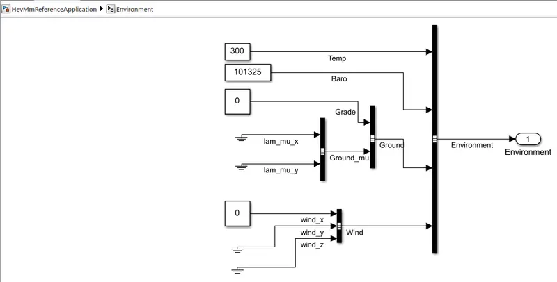
• The Grade angle = 0 degrees
• The wind velocity = 0 m/s

Result:

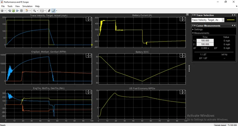
• The above figure shows the results for the simulation of Hybrid Electric Vehicle and there are totally six plots in them.
• Cursor measurement helps in understanding results in a better way.
• The cursor enables us to study the behaviour of other result parameters corresponding to the acceleration of the vehicle.

Plot 1: Trace Velocity, Target, Actual(mph)

•  It shows the velocity of the vehicle for the Drive Cycle data with the Time scale on the x-axis.
• The top speed achieved is 114 mph.
• The acceleration time to reach 114 mph is 48.687 seconds.
• The deceleration time from 114 mph to minimum is 6.061 seconds.

Plot 2: Engine Speed, Motor Speed, Generator Speed(RPM)

• It shows the changes in the speed of the engine, motor and Generator in RPM throughout the drive cycle.
• Peak Engine Speed is 5437 rpm.
• Peak Motor Speed is 13874 rpm.
• Peak Generator Speed is 5437 rpm.

 Plot 3: Engine Torque, Motor Torque, Generator Torque(Nm)

• It shows the Torque characteristics and its changes of engine, motor and generator in (Nm) throughout the drive cycle.
• Peak Engine Torque is 174 Nm.
• Peak Motor Torque is 303 Nm.

Plot 4: Battery Current (A)

• It shows the Battery Current values(A) and its changes for various acceleration inputs as per the driven cycle.
• The Peak Current Discharge from Battery is 503 A
• The Peak Current Charging to the Battery is -316 A

Plot 5: Battery SOC

• It shows the Battery State of Charge SOC(%) and its changes corresponding to the driving inputs.
• The State of Charge decreased from 80% to 61.3% of charge in 44.31 seconds for the specified driving conditions.

Plot 6: US Fuel Economy MPGe

• It shows the Fuel Economy as Miles per Gallon for the corresponding input driving conditions.
• The highest Miles per Gallon MPGe is 13.45.

 Case 2:

Simulation Condition:

• The simulation is done for Hybrid Electric Vehicle with Wide Open Throttle Drive Cycle.
• The Total Cycle Time = 100 seconds
• The Top speed of this cycle = 80 mph
• Time to start deceleration = 50 seconds
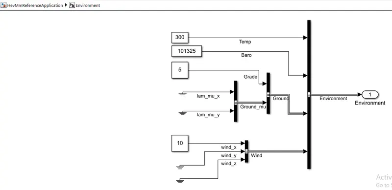
• The Grade angle = 5 degrees
• The wind velocity = 10 m/s

 

 Result:

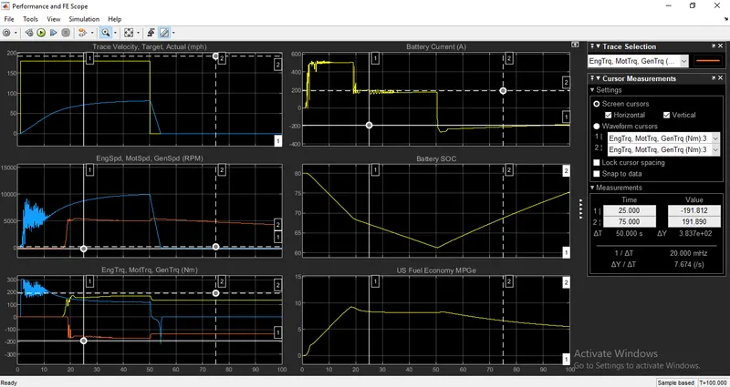
• From the above results, we can observe some changes.
• Though vehicle parameters and the drive cycle are the same, here we have considered some changes in the environment blocks by adding some hill climbing angle and wind velocity.
• The following changes in the result are given below.

Plot 1: Trace Velocity, Target, Actual(mph)

•  It shows the velocity of the vehicle for the Drive Cycle data with the Time scale on the x-axis.
• The top speed achieved is 82.42 mph.
• The acceleration time to reach 82.42 mph is 49.091 seconds.
• The deceleration time from 82.42 mph to the minimum is 16.56 seconds.

Plot 2: Engine Speed, Motor Speed, Generator Speed(RPM)

• It shows the changes in the speed of the engine, motor and Generator in RPM throughout the drive cycle.
• Peak Engine Speed is 5444 rpm.
• Peak Motor Speed is 9955 rpm.
• Peak Generator Speed is 5444 rpm.

 Plot 3: Engine Torque, Motor Torque, Generator Torque(Nm)

• It shows the Torque characteristics and its changes of engine, motor and generator in (Nm) throughout the drive cycle.
• Peak Engine Torque is 173.34 Nm.
• Peak Motor Torque is 306.64 Nm.

Plot 4: Battery Current (A)

• It shows the Battery Current values(A) and its changes for various acceleration inputs as per the driven cycle.
• The Peak Current Discharge from Battery is 520.83 A
• The Peak Current Charging to the Battery is -13.36 A

Plot 5: Battery SOC

• It shows the Battery State of Charge SOC(%) and its changes corresponding to the driving inputs.
• The State of Charge decreased from 80% to 61.38% of charge in 34.085 seconds for the specified driving conditions.

Plot 6: US Fuel Economy MPGe

• It shows the Fuel Economy as Miles per Gallon for the corresponding input driving conditions.
• The highest Miles per Gallon MPGe is 9.301.

Q4.Keeping all other parameters same, compare the simulated results of hybrid and pure electric powertrains. 

Pure Electric Vehicle: An electric vehicle (EV) is a vehicle that uses one or more electric motors or traction motors for propulsion. An electric vehicle may be powered through a collector system by electricity from off-vehicle sources, or may be self-contained with a battery, solar panels, fuel cells or an electric generator to convert fuel to electricity.EVs include, but are not limited to, road and rail vehicles, surface and underwater vessels,electric aircraft and electric spacecraft.

An example of Pure Electric car is Nissan Leaf.

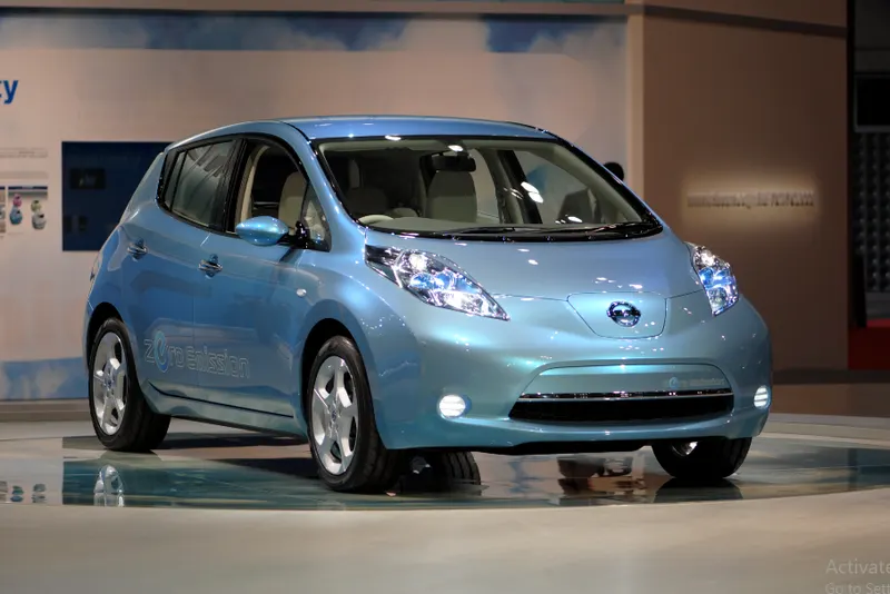
                                                                       Nissan Leaf

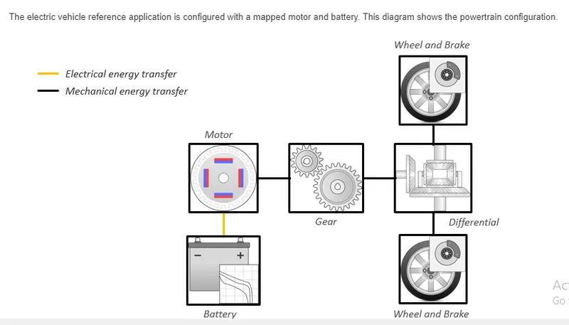
Architecture:

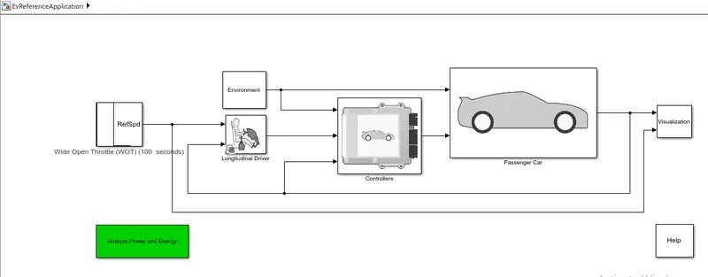
Simulation Model:

 

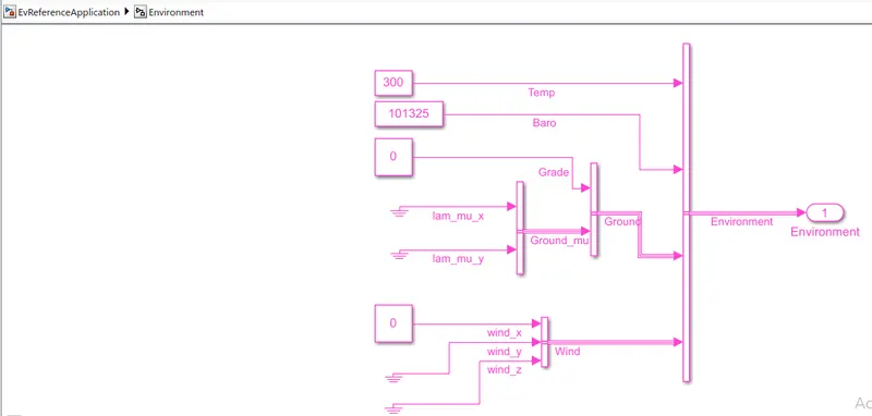
Case 1:

Simulation Condition:

• The simulation is done for Hybrid Electric Vehicle with Wide Open Throttle Drive Cycle.
• The Total Cycle Time = 100 seconds
• The Top speed of this cycle = 80 mph
• Time to start deceleration = 50 seconds
• The Grade angle = 0 degrees
• The wind velocity = 0 m/s

Result:

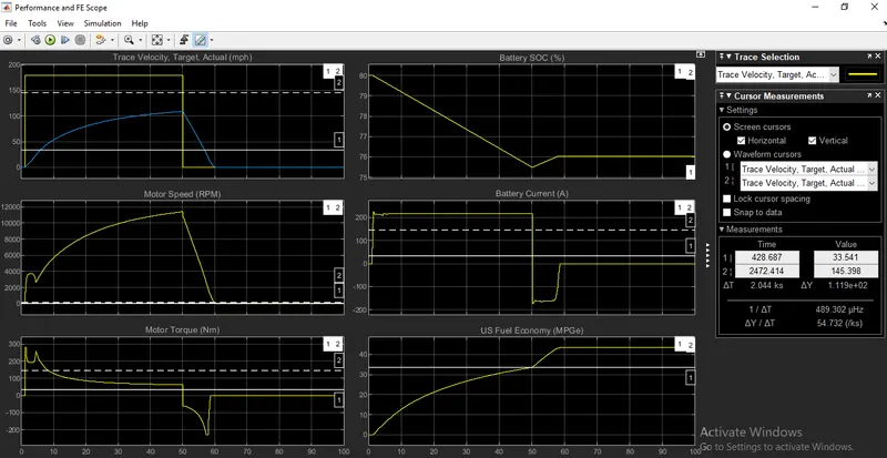
• The above figure shows the results for the simulation of Pure Electric Vehicle and there are totally six plots in them.
• Cursor measurement helps in understanding results in a better way.
• The cursor enables us to study the behaviour of other result parameters corresponding to the acceleration of the vehicle.

Plot 1: Trace Velocity, Target, Actual(mph)

•  It shows the velocity of the vehicle for the Drive Cycle data with the Time scale on the x-axis.
• The top speed achieved is 109.172 mph.
• The acceleration time to reach 109.172 mph is 48.889 seconds.
• The deceleration time from 109.172 mph to minimum is 10.505 seconds.

Plot 2: Motor Speed(RPM)

• It shows the changes in the speed of the motor in RPM throughout the drive cycle.
• Peak Motor Speed is 11409.901 rpm.

 Plot 3:  Motor Torque(Nm)

• It shows the Torque characteristics and its changes of motor in (Nm) throughout the drive cycle.
• Peak Motor Torque is 280.763 Nm.

Plot 4: Battery Current (A)

• It shows the Battery Current values(A) and its changes for various acceleration inputs as per the driven cycle.
• The Peak Current Discharge from Battery is 224.691 A
• The Peak Current Charging to the Battery is -170.752 A

Plot 5: Battery SOC

• It shows the Battery State of Charge SOC(%) and its changes corresponding to the driving inputs.
• The State of Charge decreased from 80% to 75.48% of charge in 42.914 seconds for the specified driving conditions.

Plot 6: US Fuel Economy MPGe

• It shows the Fuel Economy as Miles per Gallon for the corresponding input driving conditions.
• The highest Miles per Gallon MPGe is 43.81.

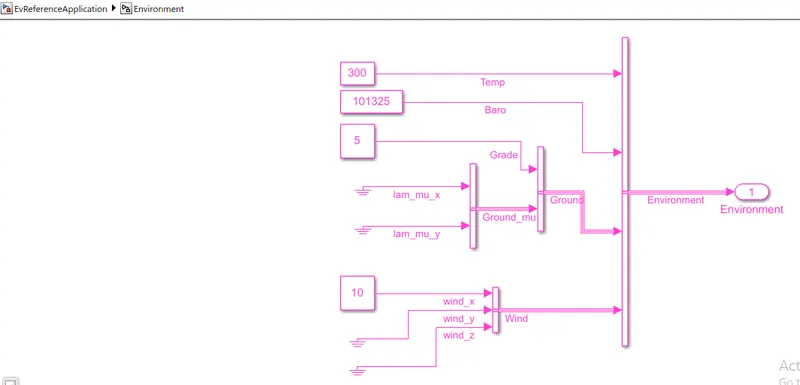
 Case 2:

Simulation Condition:

• The simulation is done for Hybrid Electric Vehicle with Wide Open Throttle Drive Cycle.
• The Total Cycle Time = 100 seconds
• The Top speed of this cycle = 80 mph
• Time to start deceleration = 50 seconds
• The Grade angle = 5 degrees
• The wind velocity = 10 m/s

 

 Result:

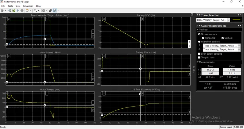
Plot 1: Trace Velocity, Target, Actual(mph)

•  It shows the velocity of the vehicle for the Drive Cycle data with the Time scale on the x-axis.
• The top speed achieved is 73.581 mph.
• The acceleration time to reach 73.581 mph is 49.697 seconds.
• The deceleration time from 73.581 mph to minimum is 6.263 seconds.

Plot 2: Motor Speed(RPM)

• It shows the changes in the speed of the motor in RPM throughout the drive cycle.
• Peak Motor Speed is 7603.341 rpm.

 Plot 3:  Motor Torque(Nm)

• It shows the Torque characteristics and its changes of motor in (Nm) throughout the drive cycle.
• Peak Motor Torque is 280.763 Nm.

Plot 4: Battery Current (A)

• It shows the Battery Current values(A) and its changes for various acceleration inputs as per the driven cycle.
• The Peak Current Discharge from Battery is 224.691 A
• The Peak Current Charging to the Battery is -162.279 A

Plot 5: Battery SOC

• It shows the Battery State of Charge SOC(%) and its changes corresponding to the driving inputs.
• The State of Charge decreased from 80% to 75.51% of charge in 15.242 seconds for the specified driving conditions.

Plot 6: US Fuel Economy MPGe

• It shows the Fuel Economy as Miles per Gallon for the corresponding input driving conditions.
• The highest Miles per Gallon MPGe is 27.565.

Conclusion:

• The Electric Vehicle when compared to hybrid electric vehicle with same environmental and Drive cycle conditions results in less top speed achievement.
• As the pure electric car here uses lithium-ion battery compared to the Nickel metal hydride battery the discharging capacity and the rate of charging is higher in the pure electric car.Also the SOC(State of Charge) shows the battery efficiency of the pure electric to be higher than the Hybrid Vehicle.
• The efficiency of the Pure Electric Car is higher than the Hybrid Elctric Vehicle which is evident from the miles per gallon numbers of both of these cars.
• Electric Vehicle produces zero emissions whereas the Hybrid Electric Vehicle produce waste gas emission. These are the some observations from the comparison of the above simulations by using Powertrain Blockset.