Week-4 Challenge WOT Condition Part-2

• What is the difference between mapped and dynamic model of engine, motor and generator?

1. Mapped Model

   Mapped Model uses a set of steady-state lookup tables to characterize engine performance. The tables provide overall engine characteristics, including actual torque, fuel flow rate, and engine-out exhaust emissions.

2. Dynamic Model

Dynamic Model decomposes the engine behavior into engine characteristics that are separated into lower-level components. By combining components in this way, the models capture the dynamic effects.

• How can you change the model type?

1. Open the Simulink window in the Matlab select the model of power train block set which is available on Matlab official website.
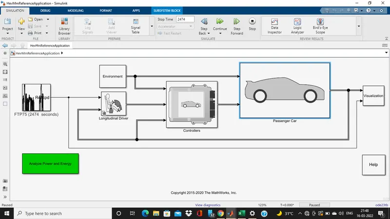
2. Select the passenger car block and double click on it.
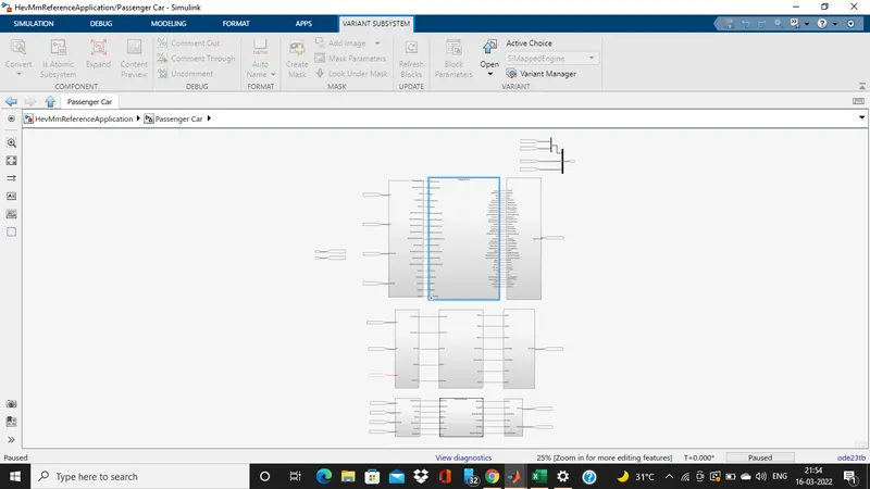
3. There you will find the engine plant already selected in the above mentioned image.
4. Above in the same window we can see the variant subsystem select this block.
5. Click on open the menu drop down and there are various options available to select one which we want.
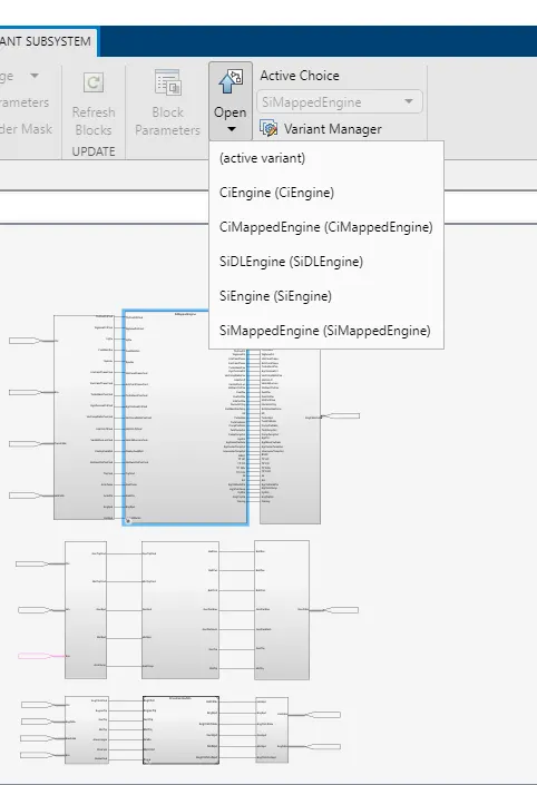
6. By this way we can switch between both the model type as per our requirement.

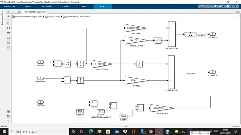
• How does the model calculate miles per gallon? Which factors are considered to model fuel flow?

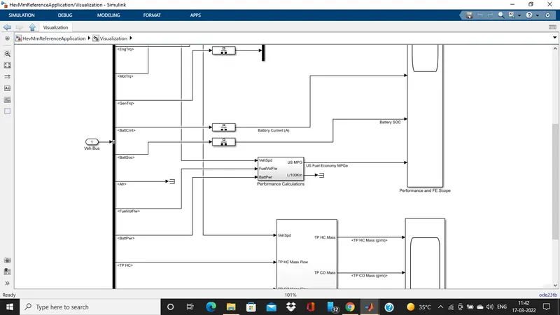
We have to open a Simulink window in the Matlab and open the reference model as mentioned in the first image. In that image we see the visualization box click on it.

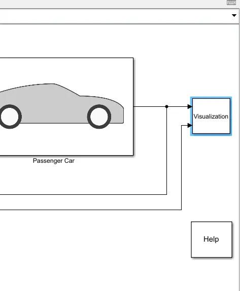
Now when we open the visualization box, we get a new window in which we can see the box name performance calculation.

When we open the performance calculation box. We got a model open which is used to calculate MPG of vehicle.

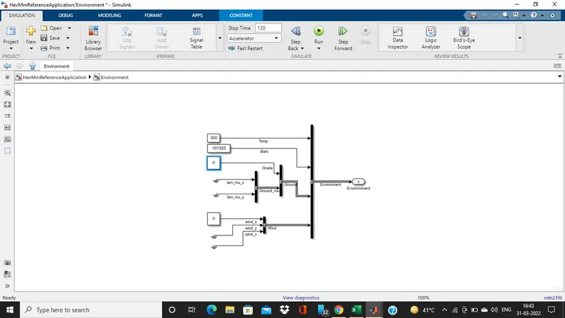
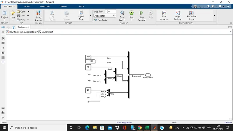
• Run the HEV ReferenceApplication with WOT drive cycle. Change the grade and wind velocity in the environment block. Comment on the results.

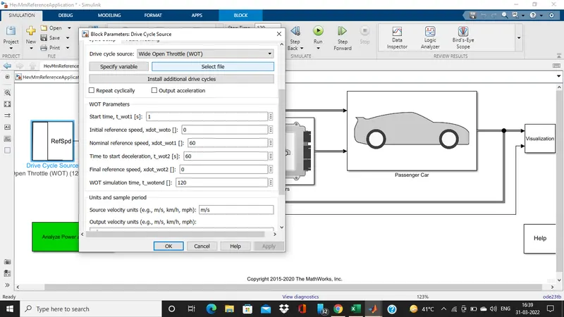
Open the hev model there we can see the Drive Cycle Source box click on it. There is a default drive cycle selected FTP 75 click on the arrow in that menu we can see the WOT (Wide Open Throttle).

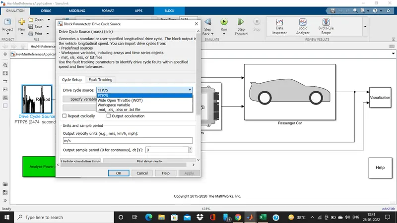
Select WOT Option and it has a default setting of 30 seconds.

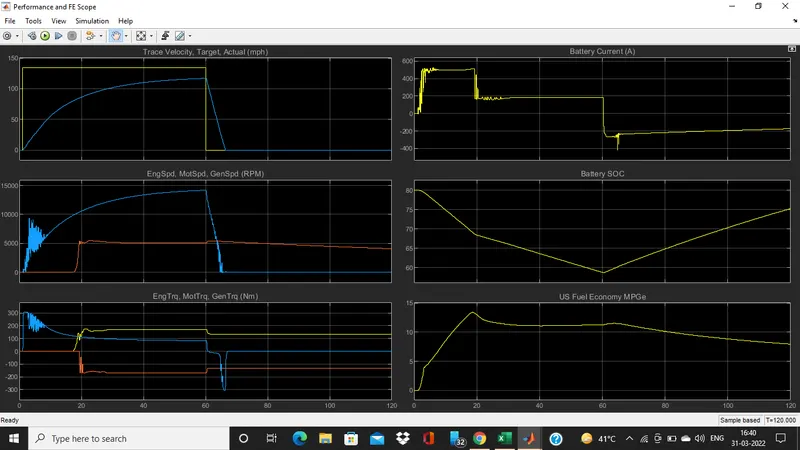
Output for default which have start time of 1 seconds, deaccelaration starts from 60 seconds, Nominal reference speed 60 seconds, WOT simulation time is 120 seconds with 0 grade and 0 wind resistance.

Output

With grade vaule of 15 and the wind resistance of 25.

Output

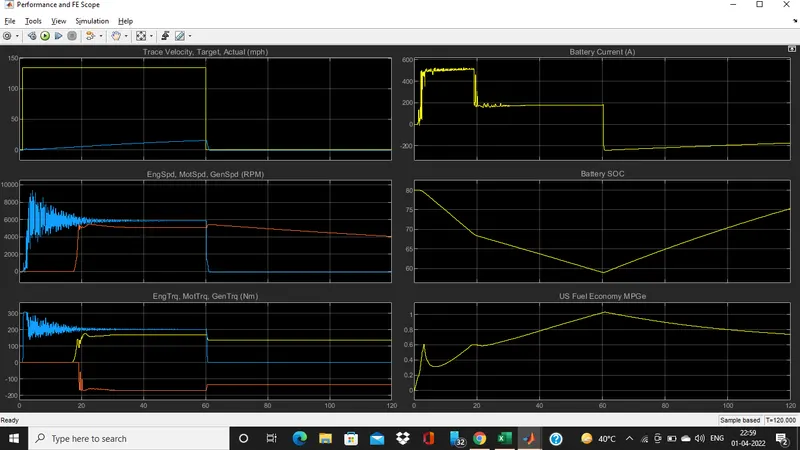
When we compare these two plots there is difference as mentioned below.

Plot 1 (Trace velocity, Target, Actual(mph)) - As we see when we add wind and grade in a setup then vehicle is not able to reach the target velocity.

Plot 2 (Engine speed, Motor speed (RPM)) - As we can see we added a grade so the speed of engine is reduced and also load of engine is increased as the previous condition and not able to reach a target speed.

Plot 3 (Engine torque, Motor torque, Generator torque(Nm)) - There are various change in these plot as we know torque is required more on the slopes as compare to flat roads.

Plot 4 (Battery current(A)) - As current required is more in second plot so there a various flacuation as compare to norml condition.

Plot 5 (Battery SOC) - In the both the condition SOC remains same variating in between 60% to 65%.

Plot 6 (Fuel Economy (MPGe)) - As we can see in the first plot the fuel economy is more as comapre to second plot.

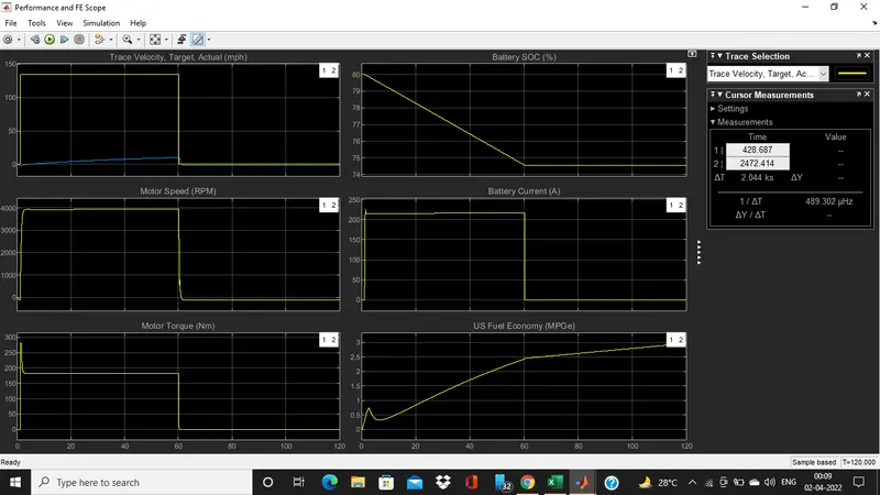
• Keeping all other parameters same, compare the simulated results of hybrid and pure electric powertrains

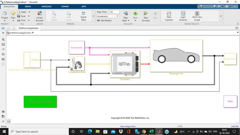
EV reference model

Output

• Reference

1. https://in.mathworks.com/help/autoblks/ug/internal-combustion-mapped-and-core-engine-models.html
2. https://in.mathworks.com/help/autoblks/ug/hev-multimode-reference-application.html