Week 4.1 - Genetic Algorithm
- Genetic Algorithms
A genetic algorithm (GA) is a method for solving both constrained and unconstrained optimization problems based on a natural selection process that mimics biological evolution. The algorithm repeatedly modifies a population of individual solutions. At each step, the genetic algorithm randomly selects individuals from the current population and uses them as parents to produce the children for the next generation. Over successive generations, the population "evolves" toward an optimal solution.
You can apply the genetic algorithm to solve problems that are not well suited for standard optimization algorithms, including problems in which the objective function is discontinuous, nondifferentiable, stochastic, or highly nonlinear.
- Working structure of genetic algorithms
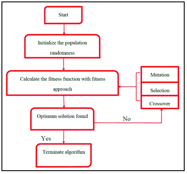
So, in the above given flowchart we see how does genetic algorithms works -
1. Population initilization - It is a very first step in the genetic algorithms. Population is a subset of solution in a current generation population (P) can also be defined as a set of chromosomes. The initial population can be generated by the two process are mentioned below
i) Random Initialization − Populate the initial population with comp-
-letely random solutions.
ii) Heuristic initialization − Populate the initial population using a kno-
-wn heuristic for the problem.
2. Selection - Selection is the stage of a genetic algorithms in which the chromosomes with the high fit-
-ness get selected.
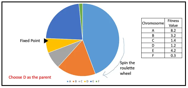
3. Crossover - It is a process of taking two parents as a solution and produce a child from them. There are many ways to do cross-over operation.
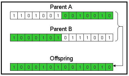
In the figure mention above one point cross-over method, where the set of genes parent A is get combimed with the parent B to create the new offspring.
4. Mutation - Mutation occur to maintain the diversitywithin the population and prevent premature
convergence.
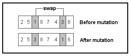
5. Fitness Function - The function which determine how fit the individual is to compete with other.
- Uses of Genetic Algorithms
Genetic Algorithms are primarily used in optimization problems of various kinds, but they are frequently used in other application areas as well. Some uses are mention below
a) Optimization − Genetic Algorithms are most commonly used in optimization problems wherein we have to maximize or minimize a given objective function value under a given set of constraints.
b) Economics − Genetic Algorithms are also used to characterize various economic models like the cobweb model, asset pricing.
c) Neural Networks − Genetic Algorithms are also used to train neural networks, particularly recurrent neural networks.
d) Image Processing − Genetic Algorithms are used for various digital image processing (DIP) tasks as well.
- Stalagmite function
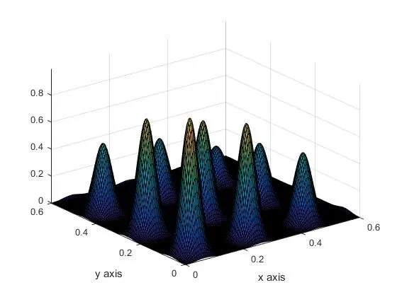
It is a mathematical model helps to gain local maxima and local minima. Stalagmite is a formation on the floor due to accumulation of material which get deposited from the ceiling drippings. It may be composed of lava, mineral, sand etc.
It is plotted as a function which is defines as -
`f(x,y) = f1x.f1y.f2x.f2y`
`f1x = (sin(5.1pix+0.5))^6`
`f1y = (sin(5.1piy+0.5))^6`
`f2x = exp[-4ln(2).(x-0.667)^2/0.64]`
`f2y = exp[-4ln(2).(y-0.667)^2/0.64]`
- Syntax of Genetic Algorithms
x = ga(fun,nvars)
x = ga(fun,nvars,A,b)
x = ga(fun,nvars,A,b,Aeq,beq)
x = ga(fun,nvars,A,b,Aeq,beq,lb,ub)
x = ga(fun,nvars,A,b,Aeq,beq,lb,ub,nonlcon)
x = ga(fun,nvars,A,b,Aeq,beq,lb,ub,nonlcon,options)
x = ga(fun,nvars,A,b,[],[],lb,ub,nonlcon,IntCon)
x = ga(fun,nvars,A,b,[],[],lb,ub,nonlcon,IntCon,options)
x = ga(problem)
[x,fval] = ga(___)
[x,fval,exitflag,output] = ga(___)
[x,fval,exitflag,output,population,scores] = ga(___)
- Matlab Program
1) Function code for genetic algorithms
function[F] = stalagmite_func(input_vector)
x = input_vector(1);
y = input_vector(2);
f1 = (sin(5.1*pi*x+0.5)).^6;
f2 = (sin(5.1*pi*y+0.5)).^6;
f3 = exp(-4*log(2)*((x-0.667).^2)/(0.64));
f4 = exp(-4*log(2)*((y-0.667).^2)/(0.64));
F = -(f1*f2*f3*f4);
end
2) Basic Program with output
%defineing our search space
x = linspace(0,0.6,150);
y = linspace(0,0.6,150);
%creating 2d mesh
[xx, yy] = meshgrid(x,y);
%evaluating the stalagmite function
for i = 1:length(xx)
for j = 1:length(yy)
input_vector(1) = xx(i,j);
input_vector(2) = yy(i,j);
f(i,j) = stalagmite_func(input_vector);
end
end
surfc(xx,yy,f)
%shading interp
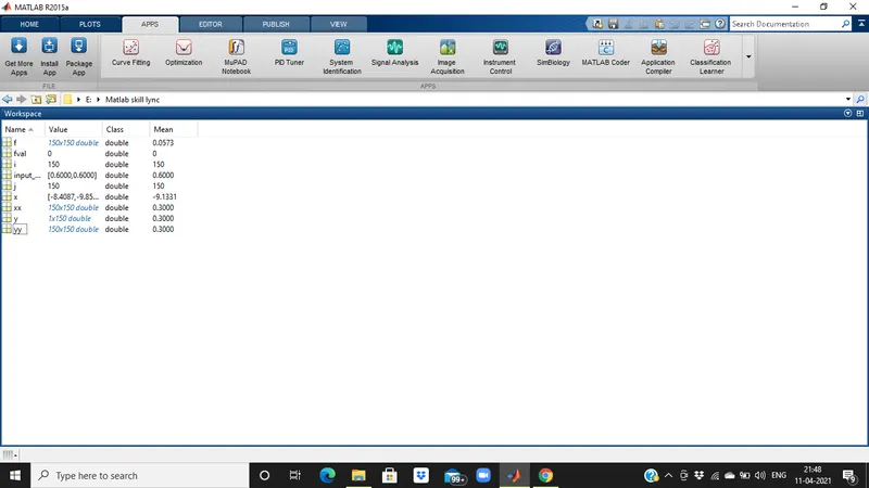
[x,fval] = ga(@stalagmite_func,2);
xlabel ('x axis')
ylabel ('y axis')
3) Program with unbounded inputs with its output
%defineing our search space
x = linspace(0,0.6,150);
y = linspace(0,0.6,150);
num_cases = 150;
%creating 2d mesh
[xx, yy] = meshgrid(x,y);
%evaluating the stalagmite function
for i = 1:length(xx)
for j = 1:length(yy)
input_vector(1) = xx(i,j);
input_vector(2) = yy(i,j);
f(i,j) = stalagmite_func(input_vector);
end
end
tic
for i=1:num_cases
[input, f(i)]=ga(@stalagmite_func,2);
x(i)=input(1);
y(i)=input(2);
end
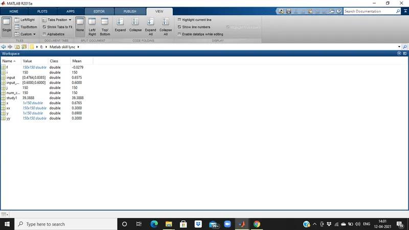
study1=toc;
figure(1)
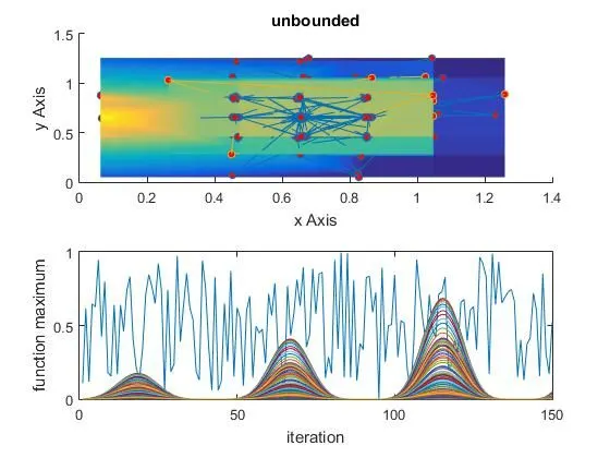
subplot(2,1,1)
hold on
surf(x,y,-f)
xlabel('x Axis')
ylabel('y Axis')
title('unbounded')
shading interp
plot3(x,y,-f,'marker','o','markersize',5,'markerfacecolor','r')
subplot(2,1,2)
plot(-f)
xlabel('iteration')
ylabel('function maximum')
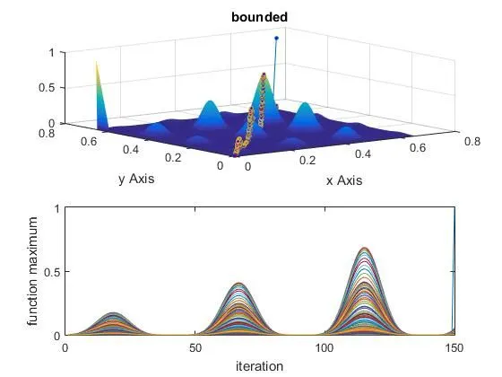
4) program with bounded inputs with its output
x = linspace(0,0.6,150);
y = linspace(0,0.6,150);
num_cases = 150;
%creating 2d mesh
[xx, yy] = meshgrid(x,y);
%evaluating the stalagmite function
for i = 1:length(xx)
for j = 1:length(yy)
input_vector(1) = xx(i,j);
input_vector(2) = yy(i,j);
f(i,j) = stalagmite_func(input_vector);
end
end
tic;
for i=num_cases
[inputs, f(i)]=ga(@stalagmite_func,2,[],[],[],[],[0;0],[1;1]);
x(i)=inputs(1);
y(i)=inputs(2);
end
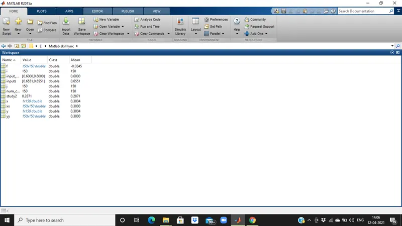
study2=toc;
figure(2)
subplot(2,1,1)
surf(x,y,-f)
shading interp
title('bounded')
xlabel('x Axis')
ylabel('y Axis')
hold on
plot3(x,y,-f,'marker','o','markersize',3,'markerfacecolor','b')
subplot(2,1,2)
plot(-f)
xlabel('iteration')
ylabel('function maximum')
5) Program with bounded inputs with increase in population with its output