Week 3 - Solving second order ODEs
ODE (odinary differential equation) is used to describe the transient behavior of a system. A simple example is a pendulum. The way in which pendulum moves depends on the Newtons second law. When the law is written we get the second order odinary differential equation the equation define the position of ball with respect to time.
Newtons second law says that the accelaration of an object is directly propotional to its force and inversely propotional to mass.
F=m.a
According to statement mention above
a=F/m
where,
a = acceleration (m/s^2)
F = Force (N)
m = mass (kg)
To write a program that solve the ode mention below. This ODE denotes the movement of pendulum.
`(d^2theta)/dt^2+b/m*(d theta)/dt+g/l*sintheta=0`
In the above equation,
g = gravity (m/s2)
L = length of the pendulum in (m)
m = mass of the ball in (kg)
b = damping coefficient.
Now, solving the above equation
`(d^2 theta)/dt^2+b/m*(d theta)/dt+g/l*sintheta`
Lets say,
`theta = theta_1`
`(d theta)/dt =theta_2`
`(d^2 ϴ)/(dt^2 ) = (d^2 theta_1)/dt^2 = d/dt((d theta_1)/dt) = (d (theta_2))/(dt)`
So, putting these assumption in above equation
`(d^2 theta_1)/dt^2 + b/m * (d theta_1)/dt + g/l*sintheta_1`
`(d theta_2)/dt + b/m*theta_2+g/l *sin theta_1`
`d/dt[[ϴ_1],[ϴ_2]] =[[theta_2],[-b/m*theta_2-g/l*sintheta_1]]`
`[[ϴ_1],[ϴ_2 ]]=theta`
Defining parameters,
Length (L) = 1m
Mass (m) = 1 kg
Gravity (g) = 9.81 m/s^2
Damping coefficient (b) = 0.05
According to given parameters i have written the matlab program which is mention below,
Function used in the program ode_func,
function [dtheta_dt] = ode_func(t,theta,b,g,l,m)
theta1 = theta(1);
theta2 = theta(2);
dtheta1_dt = theta2;
dtheta2_dt = -(b/m)*theta2 - (g/1)*sin(theta1);
dtheta_dt = [dtheta1_dt; dtheta2_dt];
end
For solving ODE,
%Second ODE
clear all
close all
clc
g = 9.81;
l = 1;
m = 1;
b = 0.05;
%initial condition
theta_0 = [0;3];
%Time
t_span = linspace(0,20,200);
%Sloving ODE
[t,results] = ode45(@(t,theta)ode_func(t,theta,b,g,l,m),t_span,theta_0);
figure(1)
plot (t,results(:,1))
hold on
plot (t,results(:,2))
xlabel ('time')
ylabel ('plot')
hold off
ct=1;
for i=1:length(t)
x0=0;
y0=0;
x1=l*sin(results(i,1));
y1=-l*cos(results(i,1));
figure(2)
plot([x0 x1],[y0 y1],'color','b')
hold on
plot([1 -1],[0 0],'color','r')
plot(x1,y1,'-','MarkerSize',50)
axis([-1 1 -1 1])
hold off
M(ct)=getframe(gcf);
ct=ct+1;
end
movie(M)
videofile = VideoWriter('Pendulum_Movement.avi','uncompressed AVI');
open(videofile)
writeVideo(videofile,M)
close(videofile)
In this above program we have used a function ode45 by thus function we can solve any high order ode which get convert into first order ode to run and then we get the results.
In the output we plotted a graph and a video of pendulum movement graph and the link of video attached below.
https://www.youtube.com/watch?v=7-xBLvBZR28&feature=youtu.be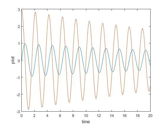
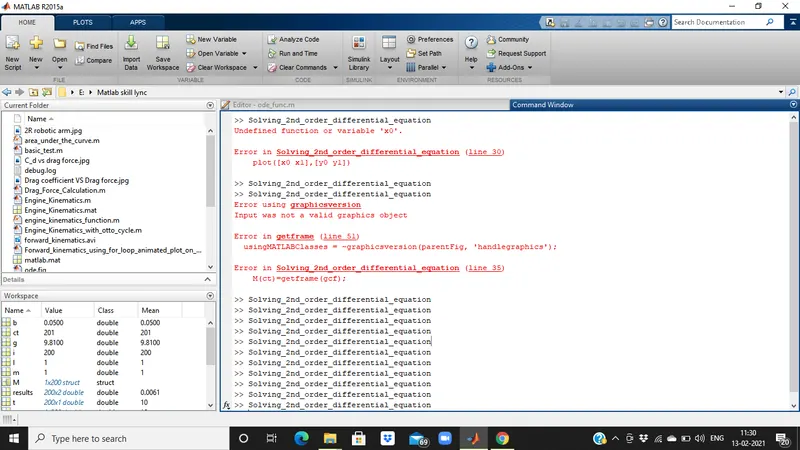
Error faced are mention below
After solving the program results are,