Week 4 - Curve fitting

Curve Fitting

• Curve fitting is a process by which we can construct a curve or mathematical function that give the best fit to a series of a data points which is possiblely subject to constraints.
• Curve fitting can involve an interpolation in which exact fit to data is required or smoothing in which a smooth function get constructed which approx fits the data.

Why do we need curve fitting?

Fitting curve can be used for an aid for data visualization to infer a values of the function where data is not available and to summrize the relationship among two or more variable.

Types of curve fitting on the basis of polynomials

Common equation used for curve fitting `y=f(x)`

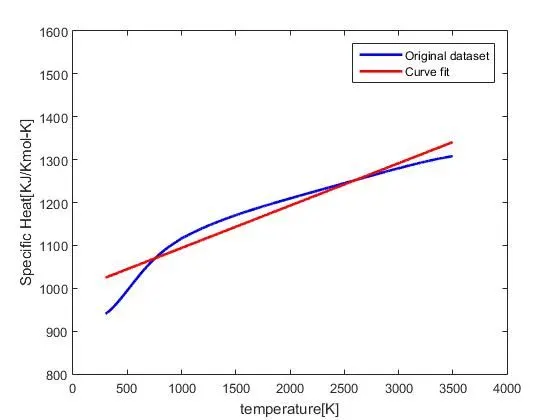
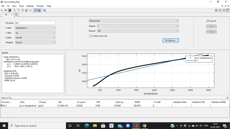
• First order polynomial equation `y = ax+b` is a line with slope a. A line can connect any two points so a first degree polynomial equation is an exact fit through any two points with distinct x coordinates.
• Second degree polynimial equation `y=ax^2+bx+c` this will fit the curve to the three points.
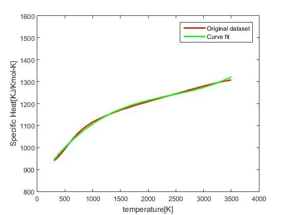
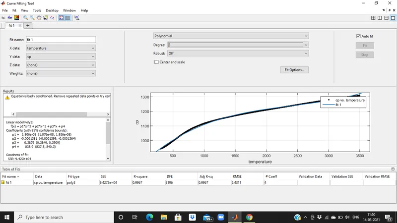
• Third degree polynomial equation `y=ax^3+bx^2+cx+d` this will fit the four points.

Parameters used to measure goodness of fit -

• The sum of square due to error (SSE)
• R-square
• Adjust R-square
• Root mean squared error (RSME)

1. The Sum of Square due to error The total deviation of the response value from the fit to response value it is also known as summed square of residuals(SSE) SSE = `sum_(i=1)^n Error i^2`
2. R-square

It is a square of a corelation between the response value and the predicted response value. It is also called square of multiple correlation and coefficient ot the coefficient of multiple determination.

Also defined as the ratio of sum of square of regression (SSR) and the total sum of square(SST).

`R^2 = (SSR)/(SST)`

SST = SSR+SSE

R-square can take any value between 0 to 1 with a value closer to 1 mean a better fit.

3. Adjust R-Square

The adjusted R-square statics can take on any value less than equal to 1, a value closer to 1 indicating a better fit.

`R_(adjusted)^2 = 1- [((1-R^2)(n-1))/(n-k-1)]`

Where, n = numbers of data ponits

k = numbers of indipendent variable

4. Root Mean squared error (RMSE)

This statisticis also known as the fit standard error and the standard error of the regression.

An RSME closer to 0 indicated a better fit.

`RMSE = sqrt((SSE)/(n))`

Perfect fit curve mean that curve should fit to original curve without any error by changing the degree of polynomial.

Code Structure

The variable get copied from the data using load command with the help of following function cp_data = load('data');

1. Each parameter in cp_data is copy to other variable i.e. cp and temperature.
2. For curve fitting of cp and temperature values so a function 'polyfit' is called and then we assigned new variable.
3. The polyfit function is used to return the coefficient in descending order of power of the polynomial and another function polyval is called and assigned a new variable.
4. These steps are used for curve fitting. The same operation are performed for a different polynomial curve fit.

Matlab Code

1. Linear Polynomial

%curve fit
%preparing data

cp_data = load('data');
temperature = cp_data(:,1);
cp = cp_data(:,2);

%Curve fit
%For first order polynomial Y=ax+b

co_effs = polyfit(temperature,cp,1);
predicted_cp = polyval(co_effs,temperature);

%compare curve fit with the original data

plot(temperature,cp,'linewidth',2,'color','b')
hold on
plot(temperature,predicted_cp,'linewidth',2,'color','r')

xlabel ('temperature[K]')
ylabel ('Specific Heat[KJ/Kmol-K]')
axis([0 4000 800 1600])
legend ('Original dataset','Curve fit')

Using Curve fitting toolbox

2. Cubic Polynomial

%curve fit
%preparing data

cp_data = load('data');
temperature = cp_data(:,1);
cp = cp_data(:,2);

%Curve fit
%For first order polynomial Y=ax^3+bx^3+cx+d

co_effs = polyfit(temperature,cp,3);
predicted_cp = polyval(co_effs,temperature);

%compare curve fit with the original data

plot(temperature,cp,'linewidth',2,'color','r')
hold on
plot(temperature,predicted_cp,'linewidth',2,'color','g')

xlabel ('temperature[K]')
ylabel ('Specific Heat[KJ/Kmol-K]')
axis([0 4000 800 1600])
legend ('Original dataset','Curve fit')

Using Curve fitting toolbox

3. Splitwise Method

%curve fit
%preparing data

cp_data = load('data');
temperature = cp_data(:,1);
cp = cp_data(:,2);

%splitting data

temperature1 = cp_data(1:800,1);
cp1 = cp_data(1:800,2);

temperature2 = cp_data(801:1600,1);
cp2 = cp_data(801:1600,2);

temperature3 = cp_data(1601:2400,1);
cp3 = cp_data(1601:2400,2);

temperature4 = cp_data(2401:3200,1);
cp4 = cp_data(2401:3200,2);

% taking cubic polynomial; y=ax+b

co_effs1 = polyfit(temperature1,cp1,3);
predicted_cp1 = polyval(co_effs1,temperature1);

co_effs2 = polyfit(temperature2,cp2,3);
predicted_cp2 = polyval(co_effs2,temperature2);

co_effs3 = polyfit(temperature3,cp3,3);
predicted_cp3 = polyval(co_effs3,temperature3);

co_effs4 = polyfit(temperature4,cp4,3);
predicted_cp4 = polyval(co_effs4,temperature4);

%plotting result

plot (temperature,cp,'linewidth',2,'color','b')
hold on
plot (temperature1,predicted_cp1,'linewidth',2,'color','g')

plot (temperature2,predicted_cp2,'linewidth',2,'color','r')

plot (temperature3,predicted_cp3,'linewidth',2,'color','y')

plot (temperature4,predicted_cp4,'linewidth',2,'color','v')
hold off

xlabel('Temperature [K]')
ylabel('Cp[KJ/K-mol K]')
axis([0 4000 800 1600])
legend ('Original dataset','Curve fit')

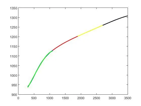
Now we get the perfect fit graph on the polynomial degree 9 and we change degree using curve fit toolbox

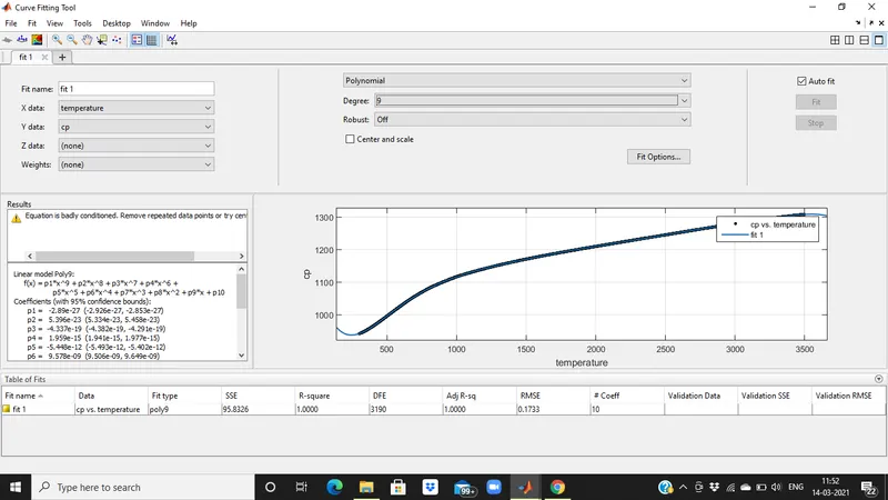
Conclusion as per the above attached graph is that accuracy of curve can increased by increase in the degree of polynomial. No as such error faced while doing this challange.

References

https://skill-lync.com/projects/Curve-Fitting-and-criterion-to-choose-best-fit-41860

https://en.wikipedia.org/wiki/Curve_fitting

http://asciimath.org/#syntax