Week 4.2: Project Transient simulation of flow over a throttle body

OBJECTIVE:

We will be performing a transient analysis on the same geometry as the previous study and document our observations as the throttle moves along with contours, plots and animations.

GEOMETRY:

We will be using the same elbow geometry:

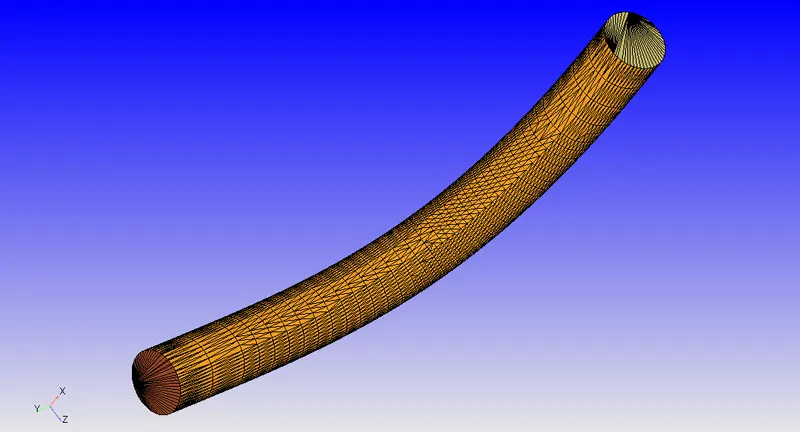
CASE SETUP:

We will be using the same case inputs, except this time we will be imparting rotating motion to the throttle:

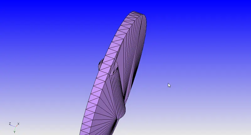
To do this, we need to calculate the coordinates of the axis of the throttle and its direction, we can see the cylindrical axis as a bulged region in the above image.

To measure the center and normal we will use the measure tool of converge:

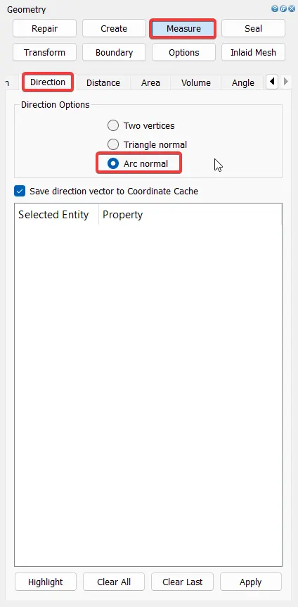
and select any three points on the arc to calculate its center and normal:

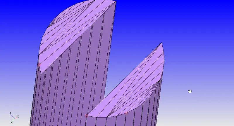
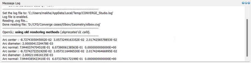
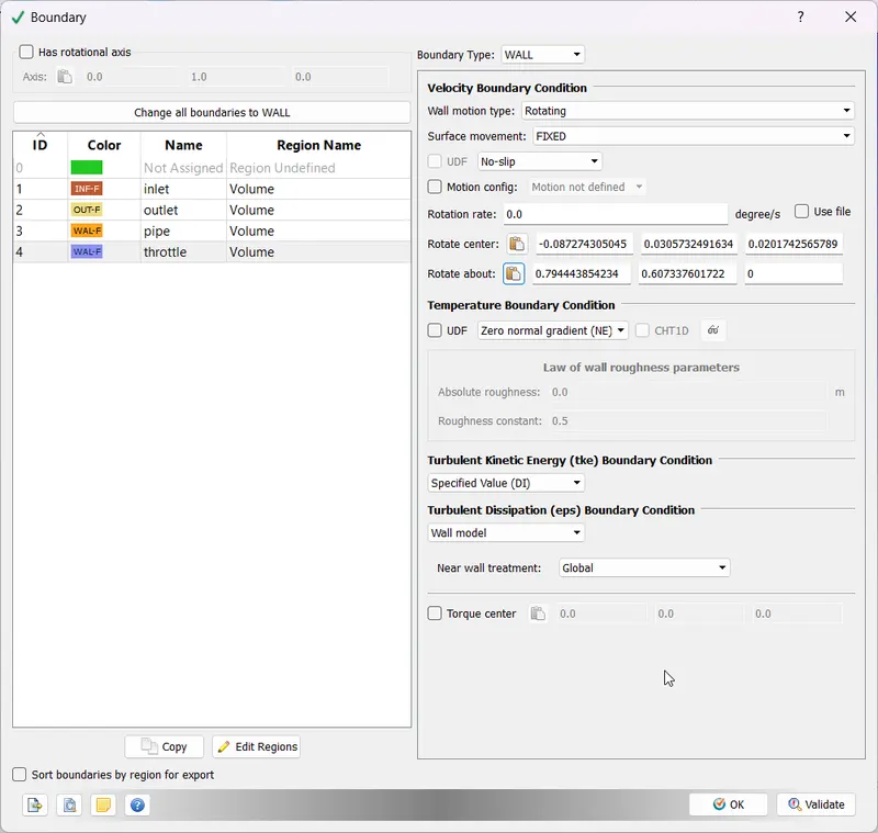
We will now copy these values and assign them as rotation centre and rotation axis in the boundary conditions and change the throttle from a stationary wall to a rotating one:

We also need to give the throttle rate of ration for which we will use a file method defined in converge:

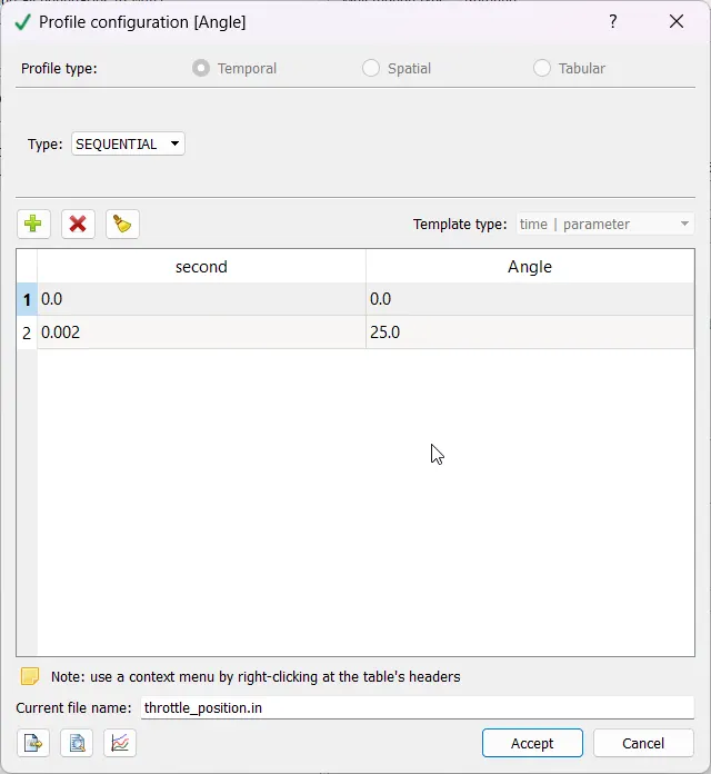
This will impart motion to the throttle rotating it by 25 degrees in 2 milliseconds, post which the position will remain constant.

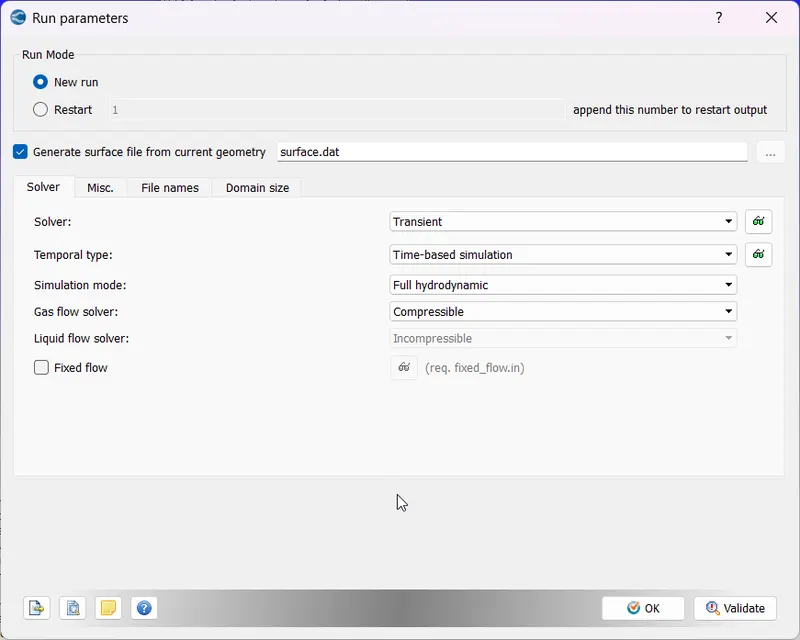
We will then change the solver to a transient one:

Next, we need to figure out the simulation end time. First, we will calculate the length of elbow using the measure tool:

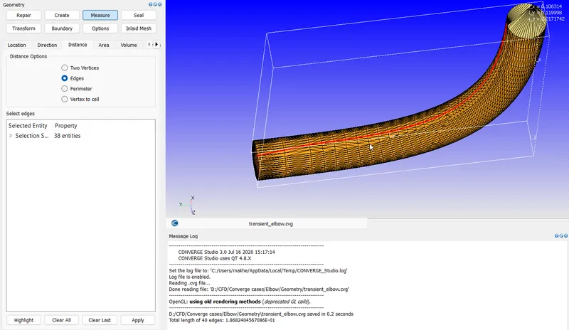
The elbow length is roughly 0.1m. In the last simulation, the average velocity was 105 m/s.
Thus, it will take the fluid approximately 1 millisecond to flow through the pipe once.

We will simulate the case 10 times that thus 10 milliseconds will be our run time to capture the results properly:

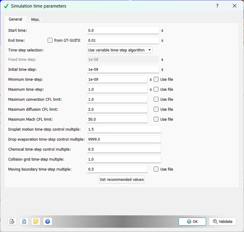
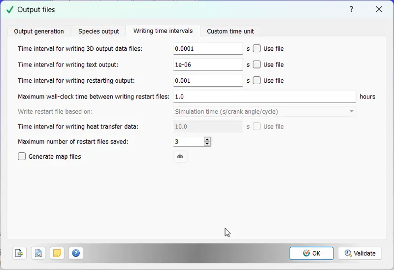
We will also change the output files writing interval so we have more files and better temporal resolution:

RESULTS:

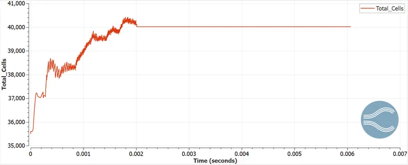
Cell count:

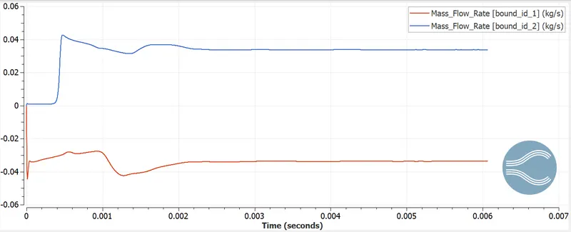
Mass Flow Rate:

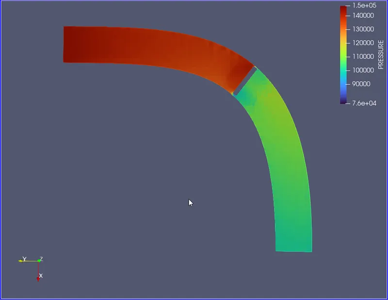
Pressure Contour:

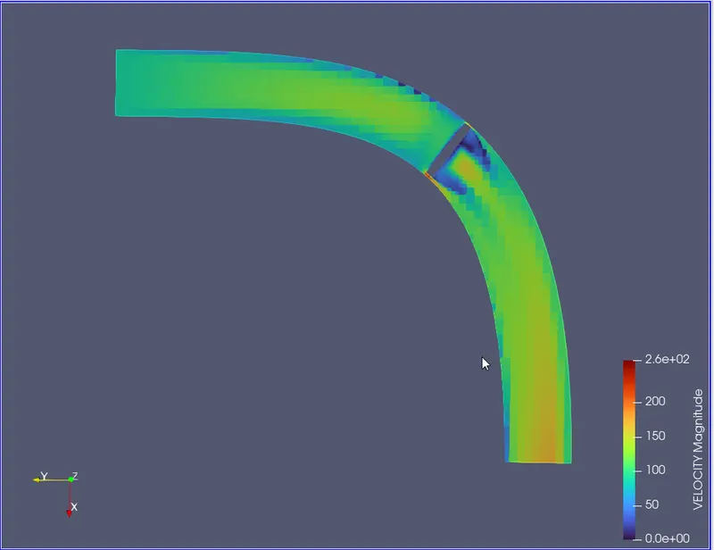
Velocity Contour:

Animations:

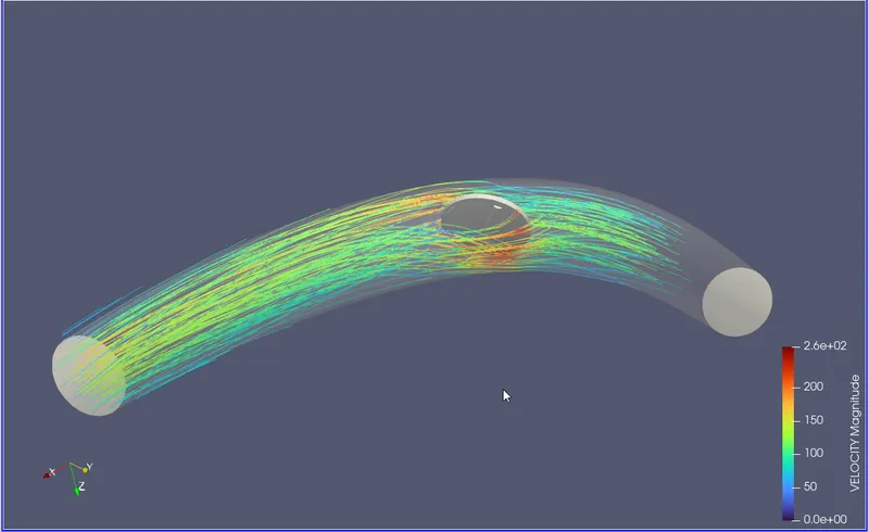
Streamline:

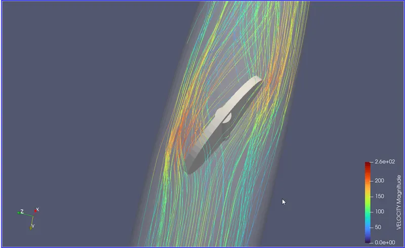
CONCLUSION:

• We see the cell count changing over time, this is due to the remeshing that occurs as the throttle moves, once the throttle stops moving the cell count becomes constant.
• We see a dip in the mass flow rate, this can be attributed to the throttle moving and closing a portion of the elbow obstructing the flow.
• In the velocity contour, we can see the region where the flow is distorted and becomes chaotic as the throttle obstructs the flow. The phenomenon can be easily observed in the streamline plot.