Week 4.1 - Genetic Algorithm
AIM - Problem Statement
To compute a set of cases with repsect to the range values with the help of Genetic Algorithm, an inbuilt function of MATLAB.
- Write a code in MATLAB to optimise the stalagmite function and find the global maxima of the function.
- Clearly expalin the concept of genetic algorithm in your own words and also explain the syntax for ga in MATLAB in your report.
- Make sure that your code gives the same output, even if it is made to run several times.
- Plot graphs for all 3 studies and for F maximum vs no. of iterations. Title and axes labels are a must, legends could be shown if necessary.
GOVERNING EQUATIONS
`f(x,y)=(f_1,x) (f_2,x) (f_1,y) (f_2,y)`
`f_1,x = [sin(5.1*pi*x+0.5)]^6`
`f_2x = exp[-4*ln(2)*(x-0.0667)^2/0.64]`
`f_1y = [sin(5.1*pi*y+0.5)]^6`
`f_2,y = exp[-4*ln(2)*(y-0.0667)^2/0.64]`
SOLUTION
Genetic Algorithm
- A genetic algorithm (GA) is a method for addressing limited and unconstrained optimization problems that is based on a natural selection process that is similar to biological evolution.
- The algorithm alters a population of individual solutions on a regular basis. At each phase, the genetic algorithm selects individuals from the present population at random to serve as parents for the following generation's children.
- The population "evolves" toward an optimal solution over generations. You can use the genetic algorithm to handle problems that aren't well suited for traditional optimization techniques, such as those with a discontinuous, nondifferentiable, stochastic, or highly nonlinear objective function.
- In two aspects, the genetic algorithm varies from a traditional, derivative-based optimization algorithm.
1. In Classical Algorithm each iteration generates a single point. The point sequence is getting closer to an ideal solution. Whereas in a Genetic Algorithm each iteration generates a population of points. The population's best point approaches an ideal solution.
2. In the classic algorithm a deterministic computation is used to choose the next point in the series. Whereas in the GA the next population is chosen by a process that employs random number generators.
Syntax of GA
1. x = ga(fun,nvars)x, to the objective function, fun. nvars is the dimension (number of design variables) of fun.
2. x = ga(fun,nvars,A,b)x to fun, subject to the linear inequalities A*x ≤ b. ga evaluates the matrix product A*x as if x is transposed (A*x').
3. x = ga(fun,nvars,A,b,Aeq,beq)x to fun, subject to the linear equalities Aeq*x = beq and A*x ≤ b. (Set A=[] and b=[] if no linear inequalities exist.) ga evaluates the matrix product Aeq*x as if x is transposed (Aeq*x').
4. x = ga(fun,nvars,A,b,Aeq,beq,lb,ub)x, so that a solution is found in the range lb ≤ x ≤ ub. (Set Aeq=[] and beq=[] if no linear equalities exist.)
5. x = ga(fun,nvars,A,b,Aeq,beq,lb,ub,nonlcon)nonlcon. The function nonlcon accepts x and returns vectors C and Ceq, representing the nonlinear inequalities and equalities respectively. ga minimizes the fun such that C(x) ≤ 0 and Ceq(x) = 0. (Set lb=[] and ub=[] if no bounds exist.)
6. x = ga(fun,nvars,A,b,Aeq,beq,lb,ub,nonlcon,options)options. (Set nonlcon=[] if no nonlinear constraints exist.) Create options using optimoptions.
7. x = ga(fun,nvars,A,b,Aeq,beq,lb,ub,nonlcon,intcon)x = ga(fun,nvars,A,b,Aeq,beq,lb,ub,nonlcon,intcon,options)intcon take integer values.
Program
First the function of stalagmite has to be defined inorder to use it in the final code;
%Defining the stalagmite function
function f=stalagmite_fun(input)
    x=input(1);
    y=input(2);
    %equation for determing the function
    f1x=(sin(((5.1*pi).*x)+0.5)).^6;
    f1y=(sin(((5.1*pi).*y)+0.5)).^6;
    f2x=exp((((x-0.0667).^2).*(-4*log(2)))./0.64);
    f2y=exp((((y-0.0667).^2).*(-4*log(2)))./0.64);

    f=-f1x*f1y*f2x*f2y;
end
The final code with details
%Genetic Algorithm(GA) in MATLAB

%Defining the search space

%The genetic algorithm doesn't know that this is the search space
%but we know that this is the search space
%X and Y are the input arrays
x=linspace(0,0.6,150);
y=linspace(0,0.6,150);
%Test case is 50
%running the program 50 times to check the accuracy of the output
num_cases=50;

%creating 2D mesh
[xx,yy]=meshgrid(x,y);
for i=1:length(xx)
   for j=1:length(yy)
       input(1)=xx(i,j);
       input(2)=yy(i,j);
       %The stalagmite function defined in another program
       %Is being called to as the value of 'f'
       f(i,j)=stalagmite_fun(input);
   end
end

%study1 - statistical behaviour of genetic algorithm
%the tic toc command
tic

for i=1:num_cases
    %Creating an optimum value that the GA will predict
%Using the stalagmite function defined in another program
    [inputs,fopt(i)]=ga(@stalagmite_fun,2);
    %x-optimum values
    xopt(i)=inputs(1);
    %y-optimum values
    yopt(i)=inputs(2);
end
%Changing the sign for a smoother plot
fopt=-fopt;
f=-f;
%The tic toc command creates the time taken for completing the GA loop
%Stores it in this studytime1,2 and 3 variable for comparing the timetaken
%For computing the studies
study1_time=toc;
figure(1);
%Subplots are used to plot two graphs inside a same window
%Easier for comparison
subplot(2,1,1);
hold on;
%This is the surface plot 3-D
%The stalagmite function
surfc(x,y,f);
shading interp;
%Plotting the x,y optimum and the optimum function values
%generated by the genetic algorithm
plot3(xopt,yopt,fopt,'marker','o','markersize',5,'markerfacecolor','b');
%title of the plots and the subplots
title('UnBounded inputs');
%The second subplot
subplot(2,1,2);
%Plotting the optimum value as a function of iteration (cases)
plot(fopt);
%X and Y labels for clear visualization
xlabel('Iterations');
ylabel('functions maxima');

%study2 statistical behaviuor with upper and lower bounds
tic
for i=1:num_cases
    %Here we are giving the upper bounds and the lower bounds
    %for a more refined data plot
    [inputs,fopt(i)]=ga(@stalagmite_fun,2,[],[],[],[],[0:0],[1:1]);
    xopt(i)=inputs(1);
    yopt(i)=inputs(2);
end
%Changing the sign for a smoother plot
fopt=-fopt;
f=-f;
study2_time = toc;
figure(2);
subplot(2,1,1);
hold on;
surfc(x,y,f);
shading interp;
plot3(xopt,yopt,fopt,'marker','o','markersize',5,'markerfacecolor','r');
title('bounded inputs');
subplot(2,1,2);
plot(fopt);
xlabel('Iterations');
ylabel('functions maxima');

%Stydy3increasing GA iteration
%giving a manual population size
%Increased population size produces refined plots
options=optimoptions('ga');
options=optimoptions(options,'PopulationSize',600);
tic
for i=1:num_cases
    [inputs,fopt(i)]=ga(@stalagmite_fun,2,[],[],[],[],[0:0],[1:1],[],[],options);
    xopt(i)=inputs(1);
    yopt(i)=inputs(2);
end
%Changing the sign for a smoother plot
fopt=-fopt;
f=-f;
study3_time=toc;
figure(3);
subplot(2,1,1);
hold on;
surfc(x,y,f);
shading interp;
plot3(xopt,yopt,fopt,'marker','o','markersize',5,'markerfacecolor','r');
title('Bounded inputs with modified population size');
subplot(2,1,2);
plot(fopt);
xlabel('Iterations');
ylabel('functions maxima');
RESULTS
The first plot shows the rather chaotic/random functions with various points, mostly unrefined points without any actual minima points.
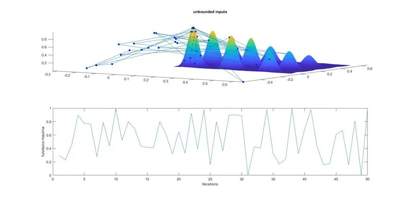
While the second study shows much more lesser values but still random, more than 14 to 15 values. In order to refine this kind of values clearly we increase the population size in study three from 150 to around 600.
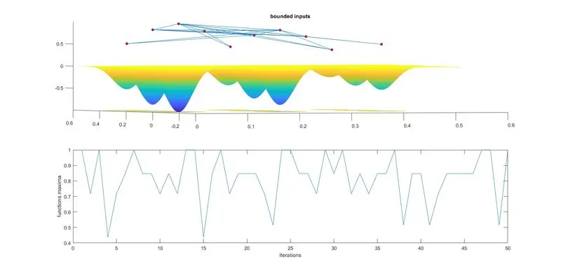
And this is the result of increasing the population size, Now we have three certain range in which the global minima will be situated.
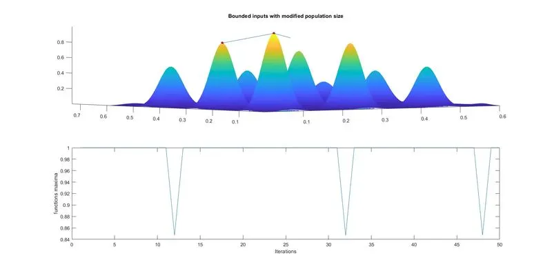
As we used the tic tok function to store the computation time of each study, we can see the difference of time when the population size is increased to 600;
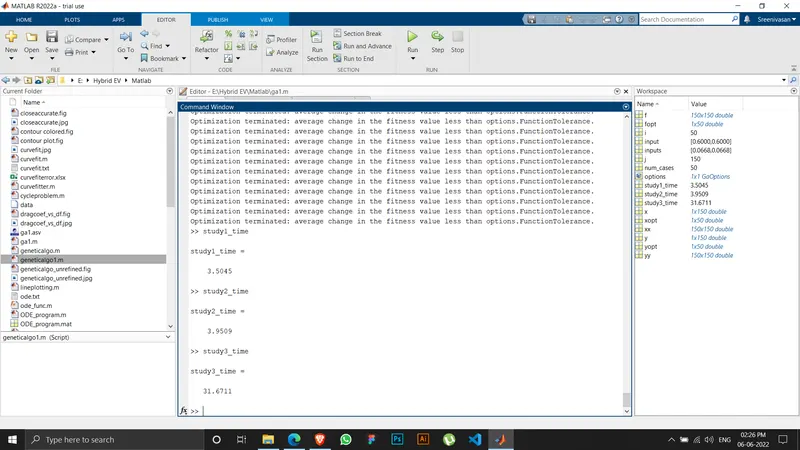
We can see that the study time 1 and 2 are almost 3 to 4 seconds while the study time 3 is a whooping 31 second. This is the drawback of increasing the population size, but only when we increase the size we get a high accuracy level.
REFERENCE
Effects of Genetic Algorithm Options - MATLAB & Simulink - MathWorks India