Week 4.1 - Genetic Algorithm

Aim: To write MATLAB code to optimise the stalagmite function and find the global maxima of the function.

Theory

Optimization is a process of finding desirable solution of a given problem which leads to the best performance under the given constraints. For example, optimization can be done in case of aero plane for its designing to reduce the drag force and to maximize the lift force for all angles of flight. In short for a given input, how desirable output can be achieved by using optimization. For all possible input’s outputs are analyzed and optimum output is selected.

Genetic algorithm (GA) is search-based optimization technique based on the principles of Genetics and natural selection. It is used to find optimum solution of complicated problem, which otherwise take very long time to solve. Whatever solutions are available, they are combined or modified to get better and better solutions. It uses techniques such as selection, mutation, inheritance, and recombination to solve problem. In genetic algorithm group of individuals is created randomly from given population. In GA population represents all possible solutions that given problem can have.

Advantages of GA

• Faster and more efficient method compared to other methods available
• It gives all possible solutions or outputs for given inputs
• It can be used to find out solution of complicated problem which otherwise takes very long time to solve.
• Useful when possible no. of solutions is very large.

Basic steps in genetic algorithm

• Start with initial population
• Selection of parent candidate’s solutions for mating.
• Crossover and mutations are applied to generate new candidate solutions.
• Determination of fitness of new candidate solution.
• Replacement of existing solution candidates with better solutions got in previous step.
• Repetition of above process till optimum solution is got.

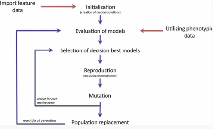
Figure: Steps inloved in GA

Genetic algorithm syntax in MATLAB

ga(@stalagmite_fun,2)

Above is the syntax to determine minimum value of a function using MATLAB. Here ‘GA’ represents genetic algorithm, stalagmite_fun is the function name and 2 represents no. of varaibales.

In general it is of the form “x = ga(fun,nvars)”.

x = ga(fun,nvars,A, b,Aeq,beq,lb,ub)

above syntax defines or specifies upper and lower bounds of a variable x so that solution will be such that x lies between upper (ub) and lower bound (lb)

MATLAB code

Function code

function f = stalagmite_fun(input)
x = input(1);
y = input(2);
f1x = (sin(((5.1*pi).*x)+0.5)).^6;
f1y = (sin(((5.1*pi).*y)+0.5)).^6;

f2x = exp((((x-0.0667).^2).*(-4*log(2)))./0.64);
f2y = exp((((y-0.0667).^2).*(-4*log(2)))./0.64);

f = -f1x*f1y*f2x*f2y;

Main code

clear all
close all
clc

%Defining search space
x = linspace(0, 0.6, 150);
y = linspace(0, 0.6, 150);
num_cases = 50;

% creating 2D mesh
[xx, yy] = meshgrid(x,y);

for i=1:length(xx)
    for j= 1:length(yy)
        input(1)=xx(i,j);
        input(2)=yy(i,j);
        f(i,j)=stalagmite_fun(input);
    end
end


% study 1 - statistical behaviour of genetic algorithm
tic
for i = 1:num_cases
    [inputs, fopt(i)] =  ga(@stalagmite_fun,2);   
    xopt(i) = inputs(1);
    yopt(i) = inputs(2);
end

fopt = -fopt
f = -f
study1_time = toc
figure(1)
subplot(2,1,1)
hold on
surfc(x,y,f)
shading interp
plot3(xopt, yopt, fopt, 'marker', 'o', 'markersize', 5, 'markerfacecolor', 'r')
title('unbounded inputs')
subplot(2,1,2)
plot(fopt)
xlabel('Iterations')
ylabel('functions maxima')


% study 2 - statistical behaviuor - with upper and lower bounds
tic
for i = 1:num_cases
     [inputs, fopt(i)] =  ga(@stalagmite_fun,2,[],[],[],[],[0:0],[1:1]);   
     xopt(i) = inputs(1);
     yopt(i) = inputs(2);
end

fopt = -fopt
f = -f

figure(2)
subplot(2,1,1)
hold on
surfc(x,y,f)
shading interp
plot3(xopt, yopt, fopt, 'marker', 'o', 'markersize', 5, 'markerfacecolor', 'r')
title('bounded inputs')
subplot(2,1,2)
plot(fopt)
xlabel('Iterations')
ylabel('functions maxima')

%Stydy 3 increasing GA iteration
options = optimoptions('ga');
options = optimoptions (options, 'PopulationSize', 500);
tic
for i = 1:num_cases
    [inputs, fopt(i)] =  ga(@stalagmite_fun,2,[],[],[],[],[0:0],[1:1], [],[],options);   
    xopt(i) = inputs(1);
    yopt(i) = inputs(2);
end

fopt = -fopt
f = -f

study3_time = toc
figure(3)
subplot(2,1,1)
hold on
surfc(x,y,f)
shading interp
plot3(xopt, yopt, fopt, 'marker', 'o', 'markersize', 5, 'markerfacecolor', 'r')
title('Bounded inputs with modified population size')
subplot(2,1,2)
plot(fopt)
xlabel('Iterations')
ylabel('functions maxima')

Results:

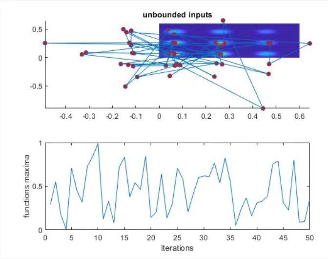
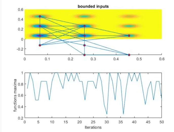
Discussion

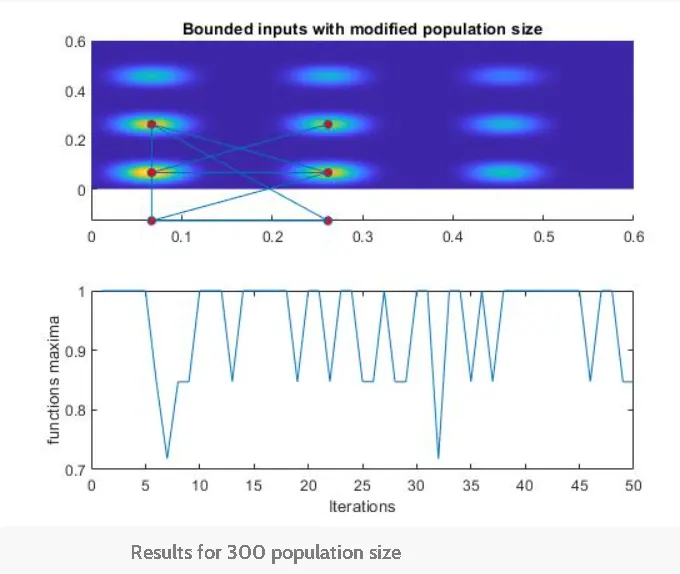
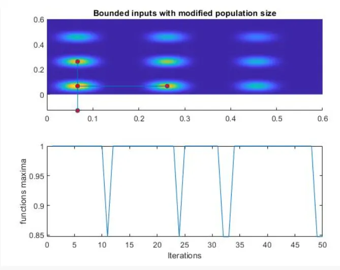
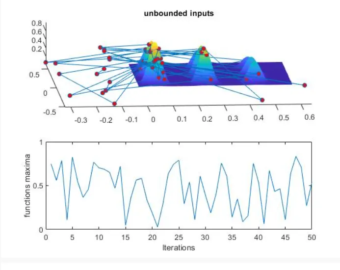
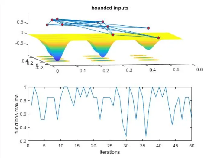
in case of unbounded inputs, the maximum values of function doesnt lies between 0 to 0.6 but is less than 0 and more than 0.6. in case of bounded inputs, the maximum values of function lies between 0 to 0.6. Also in case of bounded inputs the maximum function values is smooth and constant for atleat some iterations. With define population size, maximum function values are constant (1) except for few iterations.

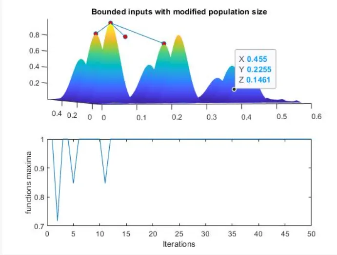
Also as population size increses there is incresed tenedency of function maximum value becomes constant as shown in figure below.