Week 3 - Solving second order ODEs

REPORT - 2nd ORDER DIFFERENTIAL EQUATION in MATLAB

Problem Statement - AIM

The aim of this challenge is to generate a plot that explains the relationship between the angular velocity and time of a pendulum hand to oscilliate in a given interval of time under the effect of acceleration due to gravity.

- Simulate the motion between 0-20 sec, for angular displacement=0,angular velocity=3 rad/sec at time t=0.

Governing Equation - The ODE equation

`(d^2theta)/dt^2 + b/m (d theta)/dt+g/L sin theta = 0`

In the above equation,

g = gravity in m/s^2,

L = length of the pendulum in m,

m = mass of the ball in kg,

b=damping coefficient dimensionless

Given values are as follows:

L=1 meter,

m=1 kg,

b=0.05.

g=9.81 m/s^2.

Program - Solution

The solution is as follows;

%Movement of a pendulum.
%2nd Order Differential Equation in MATLAB

%Inputs
%Damping ratio of the pendulum
b = 0.05;
%Acceleration due to gravity in m/s^2
g = 9.81;
%Length of the pendulum for calculation purpose in metres
L = 1;
%Mass of the pendulum in kg
m = 1;

%Initial condition for the calculation
theta_0 = [0;3];

%Time span of the pendulum and its count between the limits
t_span = linspace(0,20,200);

%solving the ODE
%Function ode_func is defined in another program and is called here
[t,results] = ode45(@(t,theta) ode_func(t,theta,b,g,L,m),t_span, theta_0);
%The ode45 command in MTALB is the differential equation solver
%ODE - Ordinary Differential Equation
%ode45 is the standard solver in MATLAB

%Plotitng the graph to see the damp and the wave
figure(1);
%Plotting the time
%Plotting the values such that all the values calculated should be plotted
plot(t,results(:,1));
hold on;
%Same goes for the angular velocity as well 
plot(t,results(:,2));
%The x-axis is time
xlabel('time');
%Y-axis is angular velocity
ylabel('angular velocity');

%Making the animation of the pendulum
figure(2);
%using the for loop for iterating and making the series of images
for i=1:length(t)
    %Creating a variable for incrementing the value of (t)
    i;
    %Plotting the x-axis base line as the frame
    %for the fixed end of the pendulum
    plot([-1.5,1.5],[0,0],'k-','LineWidth',8);
    hold on;
    %Plotting the dotted y-axis lines for reference
    plot([0,0],[0,-1.5],'k--');
    hold on;
    %Plotting the pendulum as a line
    plot([0,x(i)],[0,y(i)],'c-','LineWidth',2);
    %Plotting the pendulum ball with the use of marker function
    plot(x(i),y(i),'r-o','markersize',20,'markerfacecolor','m');
    plot(x(i),y(i),'r--');
    %Giving an axis range with the range function for better view
    axis([-1.5 1.5 -1.5 0]);
    %Pausing the frames for visibility
    pause(0.06)
    %Saving teh frames in a variable for creating a movie
    M(i)=getframe(gcf);
end
%end function for the 'for' loop
movie(M);
%Creating the movie variable to save
%this function creates the video in AVI format
videofile = VideoWriter('pendulum.avi');
%adding all the iterated frames into 1 video file.
open(videofile);
writeVideo(videofile,M);
close(videofile);

The function ode_func is defined in a new program with certain variables as discussed in the course video. The defined function was called in the main program for working.
The program is as follows:

%Defining the function ode_func for calling in the main program
function [dtheta_dt] = ode_func(t,theta,b,g,L,m)
    %Theta1 and Theta2 for completing the equation of ODE
    theta1 = theta(1);
    theta2 = theta(2);
    %This is the first order equation variant for simplified solution 
    dtheta1_dt = theta2;
    dtheta2_dt = -(b/m)*theta2 - (g/L)*sin(theta1);
    %Giving it a 1 column matrix format as it is easy to solve
    dtheta_dt = [dtheta1_dt; dtheta2_dt];

end
%End function for ending the function program

The governing equation is in the second order and so it was simplified to the first order as said by the tutor in the video.

RESULTS

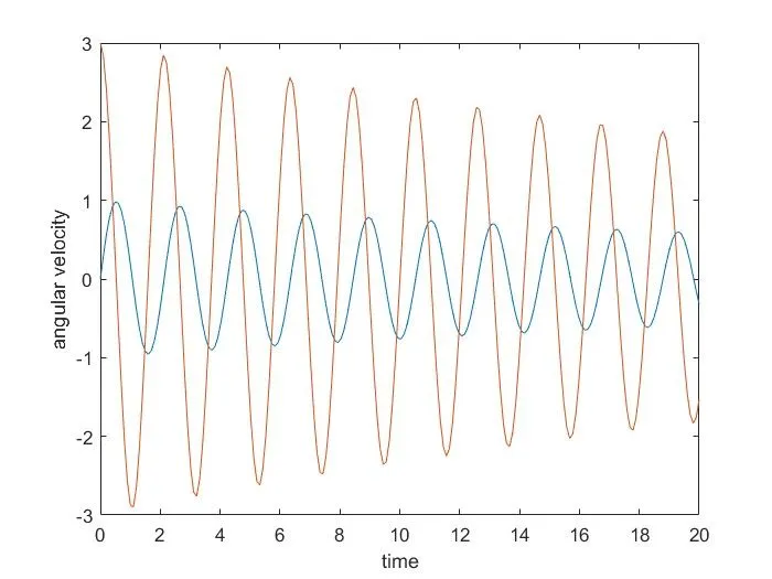
The graph showing the relation between time and angular velocity of the pendulum. In other words the graph shows each oscillation of the pendulum and the dampening of the oscillations.

CONCLUSION

There were some minor errors during the programming process as I was figuring out a way to get the for loop working, the errors are as follows:

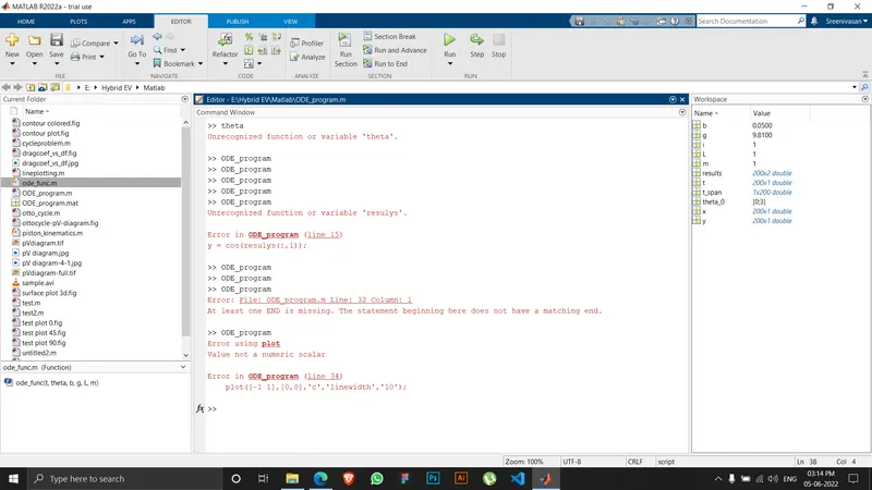
The minute errors were typos mostly and I used the help of MATLAB documentation for checking out various other interesting functions like marker, and 'r-o' which prints circles as point reference.

OUTPUT ANIMATION VIDEO
The output animated video of the file is given below via youtube link.

Youtube Video Link:

https://youtu.be/Y24QI77C3i8