Project 2 - Rankine cycle Simulator
AIM
The Ideal Rankine Cycle
The Rankine cycle is an ideal cycle for vapor power plants in which the working fluid is alternately vaporised and condensed. The term ideal implies that the cycle doesn’t involve any internal irreversibilities. The working fluid is generally water and its vapor (steam). The schematic diagram and the T-S diagram of a simple (ideal) Rankine cycle is shown in the below figure:
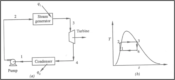
It is a thermodynamic cycle consisting of four processes namely:
1-2 - Isentropic compression in a pump
2-3 - Constant pressure or Isobaric heat addition in a boiler
3-4 - Isentropic expansion in a turbine
4-1 - Constant pressure or Isobaric heat rejection in a condenser
Process 1-2 - Isentropic compression in a pump
Water enters the pump at state 1 as saturated liquid at condenser pressure and then it is isentropically compressed to the boiler operating pressure. During this process the pump draws the energy from a prime mover, which is the work input for the cycle. Since, water is an incompressible liquid the temperature and enthalpy rise during the compression is of negligible value.
Process 2-3 - Constant pressure or Isobaric heat addition in a boiler
The compressed water from the pump enters the boiler at state2, where heat is added to it and leaves the boiler at state3. The boiler is a large heat exchanger where heat from combustion gases/nuclear reactor or other sources is used to convert the liquid water to steam at constant pressure. The boiler, together with the section where the steam is superheated (the super heater), is often called the steam generator.
Process 3-4 - Isentropic expansion in a turbine
The superheated vapor at state 3 enters the turbine, where it expands isentropically and produces work by rotating the shaft connected to an electric generator. The pressure and the temperature of steam drop during this process to the values at state 4, where steam enters the condenser.
Process 4-1 - Constant pressure or Isobaric heat rejection in a condenser
During this process, steam at saturated liquid–vapor mixture with a high quality at state 4 is condensed at constant pressure in the condenser, which is basically a large heat exchanger, by rejecting heat to a cooling medium such as a lake, a river, or the atmosphere. Steam leaves the condenser as saturated liquid and enters the pump at state1, completing the cycle.
Energy Analysis of the Ideal Rankine Cycle
The components present in the Rankine cycle (the pump, boiler, turbine, and condenser) are all steady-flow devices. Hence the cycle can be analysed using steady flow analysis. The kinetic and potential energies changes of the working fluid are very small compared to the work and heat transfer during the cycle. Hence these can be neglected.
The steady flow energy per unit mass can be written as:
`q_(In) - q_(out) + w_(In) - w_(out) = h_e - h_i [(kJ)/(Kg)]`
There is no work done in the boiler and condenser. Also, the pump and turbine are assumed to be isentropic. Then the conservation of energy relation for each device can be expressed as follows:
Pump `(q=0)`:
`w_(pump,In)= h_2-h_1 = v(p_2-p_1)`
`h_1=h_f p_1 and v~=v_1=v_f p_1`
Boiler `(w=0)`
`q_(In) = h_3-h_2`
Turbine `(q=0)`
`w_(turb,out)=h_3-h_4`
Condenser `(w=0)`
`q_(out)=h_4-h_1`
The thermal efficiency of the Rankine Cycle is determined from the equation:
`eta_(th)= w_(Net) / q_(In)`
Where, `w_(Net)= q_(In)-q_(out) =w_(turb,out)-w_(pump,In)`
The thermal efficiency can also be interpreted as the ratio of the area enclosed by the cycle on a T-S diagram to the area under the heat-addition process. The analysis of the Rankine cycle can be done using steam tables, which provide information about state properties.
OBJECTIVE OF THE PROJECT
Understand the concept of Rankine cycle by referring to standard thermal engineering text book.
- Create a Rankine Cycle Simulator using OCTAVE/MATLAB.
- Your code should calculate the state points of the Rankine Cycle (any type of your choice) based on user inputs.
- Then, plot the corresponding T-s and h-s plots for the given set of inputs. Title and axes labels are a must, while legends could be used if necessary.
- The presentation of your code will be taken into consideration while grading. Labelling sections of your code using comments is appreciated.
- Attach a report explaining the working of a rankine cycle simulator and also the research done by you.
PROGRAM
The MATLAB code is as follows:
%Basic Rankine Cycle in MATLAB
%Calculating all the outputs necessary to get the efficiency
%Data from the XSteam text file

clc;
% Description Printing for better userexperience
fprintf('Rankine Cycle \n')
fprintf('1-2 Isentropic Expansion in the turbine \n');
fprintf('2-3 constant pressure heat rejecction by the condensor \n');
fprintf('3-4 Isentropic compression in the pump \n');
fprintf('4-1 Constant pressure heat addition by the boiler \n');

% Inputs
p1=input('Enter the pressure at turbine inlet (in bar): ');
T1=input('\n Enter the Temperature at turbine inlet (in degree celcius): ');
p2=input('\n Enter the pressure at condensor inlet (in bar): ');

% calculating state point variables at each state
% state-1

% Enthalpy at pressure and Temperature 1
h1=XSteam('h_pT',p1,T1);
% Entropy at pressure and Temperature 1
s1=XSteam('s_pT',p1,T1);

%state-2

% s2=s1 because isentropic expansion
s2=s1;
% saturated liquid entropy at pressure 2
sf2=XSteam('sL_p',p2);
% saturated Vapour entropy at pressure 2
sg2=XSteam('sV_p',p2);
% Dryness fraction at state point 2
x2=(s2-sf2)/(sg2-sf2);
% saturated liquid enthalpy at pressure 2
hf2=XSteam('hL_p',p2);
% saturated Vapour enthalpy at pressure 2
hg2=XSteam('hV_p',p2);
% Enthalpy at state point 2
h2=hf2+(x2*(hg2-hf2));

%state-3

% constant Pressure at Heat Removal process
p3=p2;
% saturated liquid entropy at pressure 3
s3=XSteam('sL_p',p3);
% saturated liquid enthalpy at pressure 3
h3=XSteam('hL_p',p3);

%state-4
% Isentropic Compression Process
% constant pressure heat rejection.
s4=s3;
p4=p1;

% work done by the Turbine
W_t=h1-h2;

% work done to run pump
v3=XSteam('vL_p',p3);
W_p=v3*(p4-p3)*100;
h4=h3+W_p;

% net work
W_net=W_t-W_p;

% heat coming in to the System
Q_in=h1-h4;

% heat getting out of the system
Q_out=h2-h3;

% Thermal Effficiency
eff=(W_net/Q_in)*100;

% Back work ratio
% Ratio of pump work to turbine work
% No dimension
BWR = W_p/W_t;

% Specific steam consumption
%SSC= mass flow rate per Power
SSC=(3600/W_net);

% calculating Temperatures at state points 2,3,4
T3=XSteam('Tsat_p',p3);
T2=T3;
cp4=XSteam('cp_ps',p4,s4);
cv4=XSteam('cv_ps',p4,s4);
k=cp4/cv4;
T4=T3/((p3/p4)^((k-1)/k));

% calculating Temperature, enthalpy, entropy at Saturated vapour and liquid
T6=XSteam('Tsat_p',p1);
s5=XSteam('sL_p',p1);
s6=XSteam('sV_p',p1);
h5=XSteam('hL_p',p1);
h6=XSteam('hV_p',p1);
T5=T6;

% plotting the Saturation Curve
T=linspace(1,375,1000);
for i=1:length(T)
    % Calling the XSteam file to get
    % Saturated Liquid Entropy
    sf(i)=XSteam('sL_T',T(i));
    % Saturated Vapour Entropy
    sg(i)=XSteam('sV_T',T(i));
    % Saturated Liquid Enthalpy
    hf(i)=XSteam('hL_T',T(i));
    % Saturated Vapour Enthalpy
    hg(i)=XSteam('hV_T',T(i));
end

% plotting the T-S diagram
figure(1)
hold on
plot(sf,T,'color','r','linewidth',1)
plot(sg,T,'color','r','linewidth',1)
plot([s1 s2],[T1 T2], 'K','LineWidth',2)
plot([s2 s3],[T2 T3], 'K','LineWidth',2)
plot([s3 s4],[T3 T4], 'K','LineWidth',2)
plot([s4 s5],[T4 T5], 'K','LineWidth',2)
plot([s5 s6],[T5 T6], 'K','LineWidth',2)
sc1 =linspace(s6,s1,1000);
for l=1:length(sc1)
    Tc1(l)=XSteam('T_ps',p1,sc1(l));
end
plot(sc1,Tc1,'k','LineWidth',2)
text(s1+0.1,T1,'1')
text(s2+0.1,T2,'2')
text(s3,T3-20,'3')
text(s4,T4+20,'4')

title('Temperature Vs Entropy')
xlabel('Entropy,S (Kj/kg-k)')
ylabel('Temperture,T(Degree celcius)')
legend('Saturation Curve')

% plotting the H-S diagram

figure(2)
hold on
plot(sf,hf,'r','LineWidth',1)
plot(sg,hg,'r','LineWidth',1)
plot([s1 s2],[h1 h2], 'K','LineWidth',2)
plot([s2 s3],[h2 h3], 'K','LineWidth',2)
plot([s3 s4],[h3 h4], 'K','LineWidth',2)
hc=linspace(h4,h5,100);
for k=1:length(hc)
   sch(k)=XSteam('s_ph',p1,hc(k));
end
plot(sch,hc,'k','Linewidth',3)
plot([s5 s6],[h5 h6],'k','Linewidth',2)
for m=1:length(sc1)
    hc1(m)=XSteam('h_ps',p1,sc1(m));
end
plot(sc1,hc1,'k','LineWidth',2)
text(s1+0.1,h1,'1')
text(s2+0.1,h2,'2')
text(s3,h3-100,'3')
text(s4,h4+200,'4')
title('Enthalpy Vs Entropy')
xlabel('Entropy,S (kJ/kg-K)')
ylabel('Enthalpy,H (kJ/kg)')
legend('Saturation Curve')

% displaying results in the Command Window
disp('Results')

fprintf(('State Point-1 \n'));

fprintf('p1: %8.3f bar \n',p1);
fprintf('T1: %8.3f Deg.celcius \n',T1);
fprintf('h1: %8.3f kJ/Kg \n',h1);
fprintf('s1: %8.3f kJ/Kg-K \n',s1);


fprintf(('State Point-2 \n'));

fprintf('p2: %8.3f bar \n',p2);
fprintf('T2: %8.3f Deg.celcius \n',T2);
fprintf('h2: %8.3f kJ/Kg \n',h2);
fprintf('s2: %8.3f kJ/Kg-K \n',s2);


fprintf(('State Point-3 \n'));

fprintf('p3: %8.3f bar \n',p3);
fprintf('T3: %8.3f Deg.celcius \n',T3);
fprintf('h3: %8.3f kJ/Kg \n',h3);
fprintf('s3: %8.3f kJ/Kg-K \n',s3);


fprintf(('State Point-4 \n'));

fprintf('p4: %8.3f bar \n',p4);
fprintf('T4: %8.3f Deg.celcius \n',T4);
fprintf('h4: %8.3f kJ/Kg \n',h4);
fprintf('s4: %8.3f kJ/Kg-K \n',s4);


fprintf('Work Done by the Turbine: %8.3f kJ/Kg \n',W_t);
fprintf('Work Done by the Pump: %8.3f kJ/Kg \n',W_p);
fprintf('Net Work Done: %8.3f kJ/Kg \n',W_net);
fprintf('Efficiency: %8.3f percentage \n',eff);
fprintf('Back Work Ratio %5.1f \n', BWR);
fprintf('S.S.C:%8.3f kJ/kW \n',SSC);
RESULTS
the output of the code in the command window is shown below;
Rankine Cycle
1-2 Isentropic Expansion in the turbine
2-3 constant pressure heat rejecction by the condensor
3-4 Isentropic compression in the pump
4-1 Constant pressure heat addition by the boiler
Enter the pressure at turbine inlet (in bar): 30

 Enter the Temperature at turbine inlet (in degree celcius): 400

 Enter the pressure at condensor inlet (in bar): 0.05
Results
State Point-1
p1:   30.000 bar
T1:  400.000 Deg.celcius
h1: 3231.571 kJ/Kg
s1:    6.923 kJ/Kg-K
State Point-2
p2:    0.050 bar
T2:   32.875 Deg.celcius
h2: 2110.708 kJ/Kg
s2:    6.923 kJ/Kg-K
State Point-3
p3:    0.050 bar
T3:   32.875 Deg.celcius
h3:  137.765 kJ/Kg
s3:    0.476 kJ/Kg-K
State Point-4
p4:   30.000 bar
T4:   36.935 Deg.celcius
h4:  140.776 kJ/Kg
s4:    0.476 kJ/Kg-K
Work Done by the Turbine: 1120.863 kJ/Kg
Work Done by the Pump:    3.011 kJ/Kg
Net Work Done: 1117.852 kJ/Kg
Efficiency:   36.167 percentage
Back Work Ratio   0.0
S.S.C:   3.220 kJ/kW
The output plots are shown below;
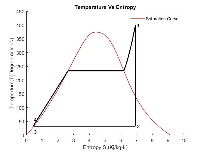
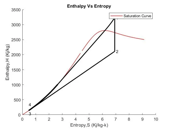
CONCLUSION
Required Inputs:
Turbine Inlet temperature = 400° C
Turbine Inlet Pressure = 30 bars
Turbine Outlet Pressure = 0.05 bars = Condenser Inlet Pressure
The program successfully executed the above input and the values are printed in the command window with expected results.
The following outputs were successfully calculated
- Net work output
- Back work ratio
REFERENCE
1. Ideal Rankine Cycle (iitk.ac.in)