Week 4.1 - Genetic Algorithm

[x,fval,exitflag,output,population,scores] = ga(___)

2. Reference has taken for the code and the understanding of the GA function by the below link:-
> https://www.researchgate.net/profile/Manish-Saraswat/publication/258789666_Optimization_of_Function_by_using_a_New_MATLAB_based_Genetic_Algorithm_Procedure/links/5d368b51a6fdcc370a577ffd/Optimization-of-Function-by-using-a-New-MATLAB-based-Genetic-Algorithm-Procedure.pdf

>Doc ga: Inbuild document for GA.

#Main Code:

close all 
clear all
clc

%Assigning values to x and y

x= linspace(0,0.5,150);
y= linspace(0,0.5,150);
range= 50;

% Making a 2D mesh
[xx, yy]= meshgrid(x,y);

for i=1:length(xx) 
    for j=1:length(yy)
        input(1)= xx(i,j);
        input(2)= yy(i,j);
        h(i,j)= stalagmite_func(input);
    end
end

%Case 1: The Ga function without upper and lower bounds:-
tic
for i= 1:range
    [inputs, dopt(i)]= ga(@stalagmite_func, 2);
    xopt(i)=inputs(1);
    yopt(i)=inputs(2);
end

%To get the maximum value out of the Stalgamite function
dopt= -dopt;
h=-h;
study_1= toc;

%Plotting the Graph
figure(1)
subplot(2,1,1)
%hold on
%To get the surface smooth and remove grid lines
surfc(x,y,h)
shading interp
hold on
plot3(xopt, yopt, dopt,'Marker','o','MarkerFaceColor','r','MarkerSize',15,'MarkerEdgeColor','b');
title('Unbounded points')
subplot(2,1,2)
plot(dopt)
%To label the axes
xlabel('Iteration')
ylabel('functions maxima')

%Case 2: Defining the upper and lower bound in the GA function:-

tic
for i= 1:range
    [inputs, dopt(i)]= ga(@stalagmite_func, 2,[],[],[],[],[0,0],[1,1]);
    xopt(i)=inputs(1);
    yopt(i)=inputs(2);
end

%To get the maximum value out of the Stalgamite function
dopt= -dopt;
h=-h;
study_2= toc;

%Plotting the Graph
figure(2)
subplot(2,1,1)
%hold on          % To show all the instances
%To get the surface smooth and remove grid lines
surfc(x,y,h)
shading interp
hold on   
plot3(xopt, yopt, dopt,'Marker','o','MarkerFaceColor','r','MarkerSize',15,'MarkerEdgeColor','b');
title('Maximum points')
subplot(2,1,2)
plot(dopt)
%To label the axes
xlabel('Iteration')
ylabel('functions maxima')
%Case 2: Defining the upper and lower bound in the GA function:-

tic
for i= 1:range
    [inputs, dopt(i)]= ga(@stalagmite_func, 2,[],[],[],[],[0,0],[1,1]);
    xopt(i)=inputs(1);
    yopt(i)=inputs(2);
end

%To get the maximum value out of the Stalgamite function
dopt= -dopt;
h=-h;
study_2= toc;

%Plotting the Graph
figure(2)
subplot(2,1,1)
%hold on          % To show all the instances
%To get the surface smooth and remove grid lines
surfc(x,y,h)
shading interp
hold on   
plot3(xopt, yopt, dopt,'Marker','o','MarkerFaceColor','r','MarkerSize',15,'MarkerEdgeColor','b');
title('Maximum points')
subplot(2,1,2)
plot(dopt)
%To label the axes
xlabel('Iteration')
ylabel('functions maxima')

% Case 3: Defining the population to be observed with upper and lower bound

%Using'ga' function and optimization:-

options= optimoptions('ga');
options= optimoptions(options, 'PopulationSize',200);

tic
for i= 1:range
    [inputs, dopt(i)]= ga(@stalagmite_func, 2,[],[],[],[],[0,0],[1,1],[],[],options);
    xopt(i)=inputs(1);
    yopt(i)=inputs(2);
end

%To get the maximum value out of the Stalgamite function
dopt= -dopt;
h=-h;
study_3= toc;

%Plotting the Graph
figure(3)
subplot(2,1,1)
%hold on             % To show all the instances
%To get the surface smooth and remove grid lines
surfc(x,y,h)
shading interp    
hold on
plot3(xopt, yopt, dopt,'Marker','o','MarkerFaceColor','r','MarkerSize',15,'MarkerEdgeColor','b');
title('Maximum points')
subplot(2,1,2)
plot(dopt)
%To label the axes
xlabel('Iteration')
ylabel('functions maxima')
xlabel('Iteration')
ylabel('functions maxima')



% Case 3: Defining the population to be observed with upper and lower bound

%Using'ga' function and optimization:-

options= optimoptions('ga');
options= optimoptions(options, 'PopulationSize',200);

tic
for i= 1:range
    [inputs, dopt(i)]= ga(@stalagmite_func, 2,[],[],[],[],[0,0],[1,1],[],[],options);
    xopt(i)=inputs(1);
    yopt(i)=inputs(2);
end

%To get the maximum value out of the Stalgamite function
dopt= -dopt;
h=-h;
study_3= toc;

%Plotting the Graph
figure(3)
subplot(2,1,1)
%hold on             % To show all the instances
%To get the surface smooth and remove grid lines
surfc(x,y,h)
shading interp    
hold on
plot3(xopt, yopt, dopt,'Marker','o','MarkerFaceColor','r','MarkerSize',15,'MarkerEdgeColor','b');
title('Maximum points')
subplot(2,1,2)
plot(dopt)
%To label the axes
xlabel('Iteration')
ylabel('functions maxima')
xlabel('Iteration')
ylabel('functions maxima')



​

#Supporting Code:-

function st= stalagmite_func(input_vector)

a=input_vector(1);
b=input_vector(2);
t1=(sin(((5.1*pi).*a) + 0.5)).^6;
t2=exp((((a-0.0667).^2).*(-4*log(2)))./0.64);
t3=(sin(((5.1*pi).*b) + 0.5)).^6;
t4=exp((((b-0.0667).^2).*(-4*log(2)))./0.64);

st=-(t1*t2*t3*t4);

end

#Output:-

The Stalagmite function:-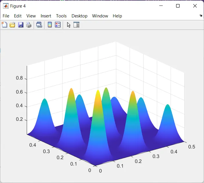



Case1: GA function without optimization and unbounded.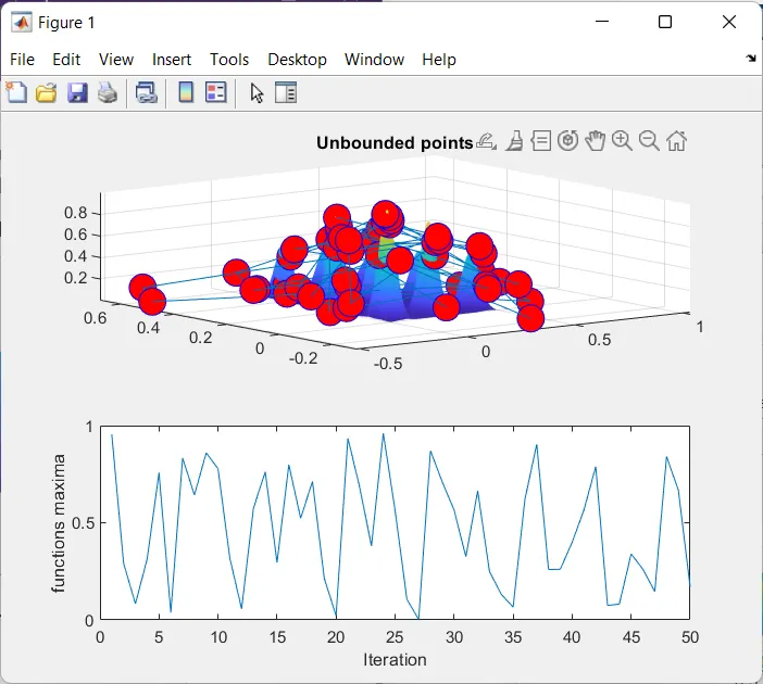



Case 2: Ga function with upper and lower bound.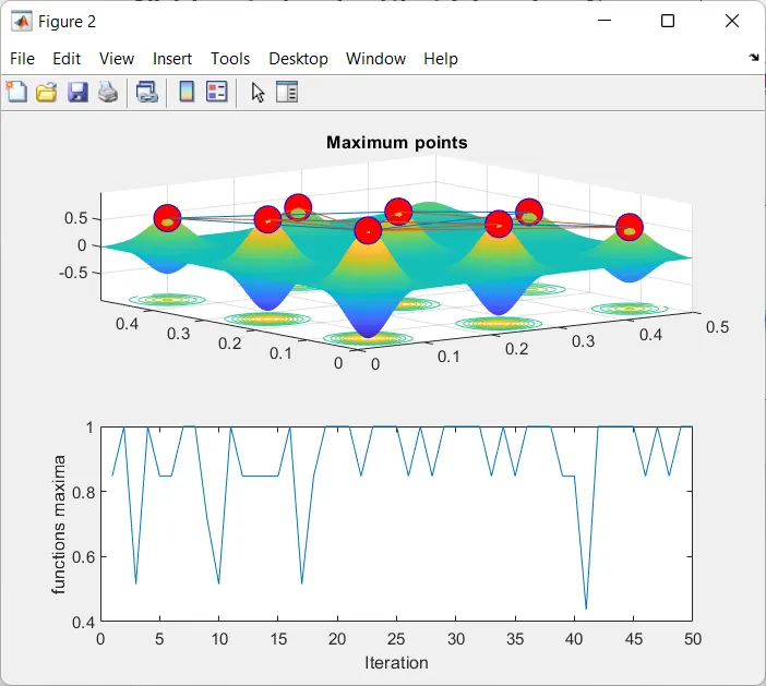




Case 3: GA function with optimization and upper and lower bounds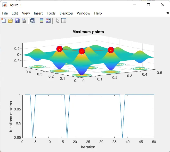





#Code Explanation:-

> At first we initialize the variables using linspace commande to create 150 values between the initial and final value.

> Then we create a 2d mesh using the 'meshgrid' command and introduce another variable to set the range upto 50.

> Now, we have created a loop in order to call our stalagmite function and initialize its inputs.

> Parallely, we have also created a supported function for stalagmite function called "stalagmite_func", which is defined as :-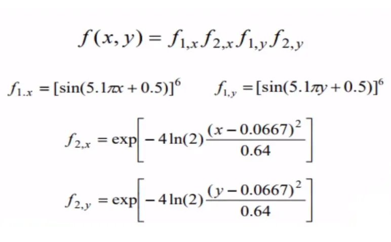



> Then, we start with our first case without setting the upper and lower bound of the GA function, thus using the syntax
"ga(@stalagmite_func, 2);" and getting a vague arbitrary output.

>After which we use the command 'surfc' and 'shading interp' command to show the surface of the curve and remove the gridlines and get a smooth curve after which we plot the first curve.

>Now, we move on to the next case and provide the GA function with the necessary upper and lower bound thjus using the suntax '[inputs, dopt(i)]= ga(@stalagmite_func, 2,[],[],[],[],[0,0],[1,1]);'

>And then we follow the same procedure to get the plot for the next case, case 2.

>Then we move on to the final case, and optimise our solution even move by setting the population range and using the 'optimoption' command to refine our output.

Note: In the code case 2 and case 3 are taken twice to get the upper bound of the cases correctly according to the given plot.

#Errors Faced:-

>> We needed to add the 'hold on' command in order to show the previous instances of the plot.
> We need to check for the syntax of the Ga command and select it according to our parameters otherwise you will get an error, to remove it and know about the syntax, we refer to the 'doc ga' command in the command window.

#Conclusion:-

>>GA function has a large scope in the field where data needs to be saturated and has many uncertainties.