Week 3 - Solving second order ODEs

Aim: To write a program in Matlab that will solve an ODE and simulate the result in a pendulum motion having a damping effect.

Equation involved:-

In the above equation,

g = gravity in m/s2,

L = length of the pendulum in m,

m = mass of the ball in kg,

b=damping coefficient.

Default values are taken in the code:-

L=1 metre,

m=1 kg,

b=0.05.

g=9.81 m/s2.

time = 0-20 seconds

initial angular velocity= 3 m/s^2

initial angular displacement= 0 rad


Youtube Link: https://youtu.be/co4KyNkKcUw


#Main Code:-

%Code for solving 2nd order differential equation:-
clc
close all
clear all

l=1;                 %in meter
m=1;                 %in Kgs
b=0.05;
g=9.81;              %in m/s^2

%Initital condition

theta_0= [0;3];

%Time Specifications

t1= linspace(0,20,500);      %time from 0-20 sec having 500 values in between

%solving the ode

[t, results]= ode45(@(t,theta) ode_func(t,theta,b,g,l,m),t1,theta_0);

x0=0;                       %Hinge coordinates
y0=0;
plot(x0,y0,'marker','+');   %Plotting the Hinge
y=results(:,1);             %seperating the displacement column from above results
ct=1;                       %initializing counter variable
for i=1:length(t1)
    
    x1=l*sin(y(i));
    y1=-l*cos(y(i));        %negative since we are dealing with values below zero
    plot([x0 x1],[y0 y1], "Marker","*",'MarkerFaceColor','b',"MarkerSize",15,"MarkerEdgeColor","r");
    hold on                 %To show all the instances
    plot(x1, y1, "Marker","o",'MarkerFaceColor','r',"MarkerSize",15,"MarkerEdgeColor","b");
    hold off                %To erase the previous instances so transition looks smooth
    title('Simple harmonic motion');
    ylabel('Displacement');    %Labelling the x and y coordinates
    xlabel('Time');
    axis([-1 1 -2 0]);         %setting limits 
    R(ct)=getframe(gcf);       %for capturing the resulting of this iteration
    pause(0.02);
    ct=ct+1;

    
end
movie(R);                       %for showing the captured images of the above loop
videofile=VideoWriter('ODE_Pendulum.avi','Uncompressed AVI');
open(videofile)
writeVideo(videofile,R)
close(videofile)

#Supporting Function Code:-

function[dtheta_dt]= ode_func(t,theta,b,g,l,m)
theta1=theta(1);
theta2=theta(2);
dtheta1_dt=theta2;
dtheta2_dt=-(b/m)*theta2-(g/l)*sin(theta1);
dtheta_dt=[dtheta1_dt;dtheta2_dt];
end

Result:-
Note: The below result is just one instance, to see the entire result kindly refer to the youtube link or run the code.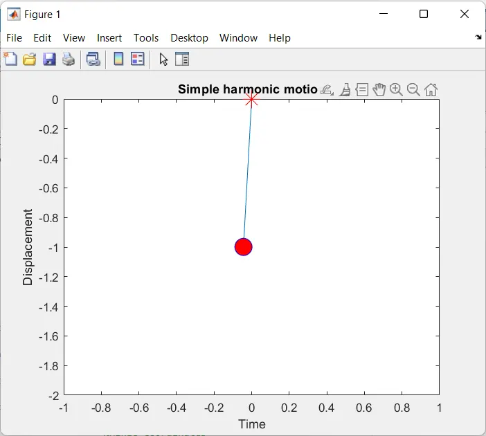



Code Explanation:-

> At first we initialize the default values of the code, namely, l, m, b, etc. Afterwhich we then use an array to initialize the displacement and velocity values.

> Now, with using the function 'linspace' to create equal instances, we set the range of time from 0-20 sec having 500 instances in between.

>Then we create the supporting function to set the operations of the ODE we wanted to solve by the equation below and put its value in a function called 'ode_func':-

dtheta2_dt=-(b/m)*theta2-(g/l)*sin(theta1)

> Now we call the above function and use the in-built Matlab function called 'Ode45' to solve our differential equation and put its values in 'results'.

> Now we set the coordinates for the hinge and plot it. Followed by, separating the values of displacement in a separate variable called 'y' and initializing the counter variable for our upcoming loop.

> We, then start a loop that runs for the length of values that the time has, in which we initialize the coordinates of the string and the pendulum mass using simple trigonometric equations and plot them accordingly.

> We also use the 'Hold on' and 'Hold off' commands to show all the instances smoothly, and we use the 'marker' command to create a circle at the end of the string to visualize the mass even better.

>Then we give our plot a name using the 'title' command and followed by ging the name to the axis of the plot.

>Now, we set the limit of our plot using the axis command.

> Then we use the 'getframe' command to capture the output generated by the loop following which we have incremented our counter variable.

>Now with the movie command we show all the instances in an animation, following which we save the animation and generate an '.avi' file by creating a file object called 'videofile', by opening it, writing in it and clsing it.

Errors Faced:-


#1: Here we need to add the 'Hold Off' command in order to erase the previous instances or we will get the below result:-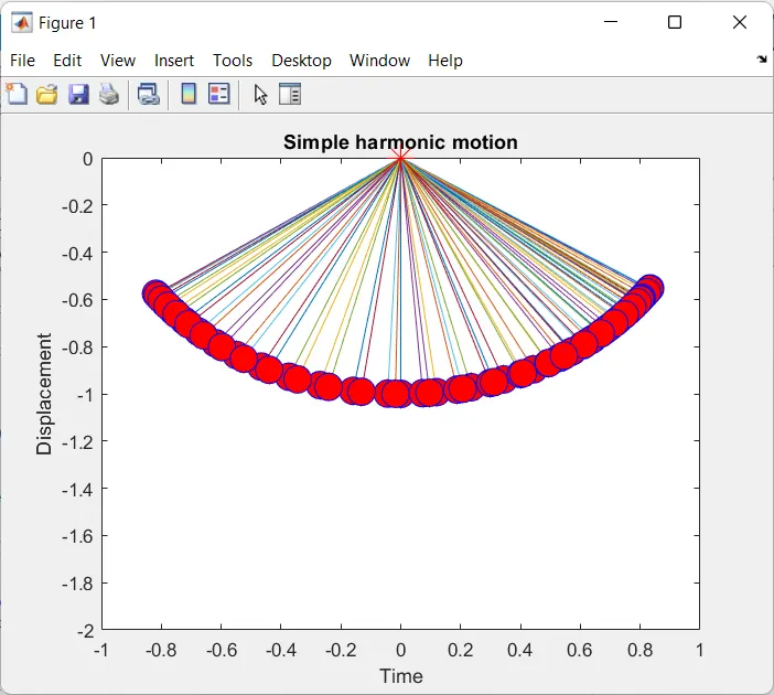



#2: Adding the get frame function after the increment of the variable called 'ct'. This results in not showing the first figure frame captured by ct, as that frame was not recorded, thereby starting of the output when ct has already reached a value of 2.
Hence ct needed to be incremented at the very last of the second loop so that the first image will get captured and recorded.

Conclusion:-

> Using the Matlab ODE45 function and plotting the result, we can visualize the damping effect on a pendulum even more clearly.