Week 4.1 - Genetic Algorithm
AIM:
Write a code MATLAB to optimise stalagmite function and find the global maxima genetic algorithm.
OBJECTIVES:
Clearly explain the concept of the GENETIC ALGORITHM in your words and ga of the syntax.
Make sure your code gives same outputs ,even it may run several times runs.
GENETIC ALGORITHM CONCEPT:
The genetic algorithm is an algorithm used both constrained and unconstrained optimization problems.
The genetic alorithm is maximum and minimum values to find.
A genetic algorithm is a search heuristic that is inspired by Charles Darwin's theory of natural evolution.
It selects random inputs called as population ,check their fitness for selection and pairing purposes,
to generate new data.
This next generation data is mutated from data aquired from parents which is essential for computing
optimised output.
The genetic algorithm uses three main types of rules at each step to create the next generation from the
current population.
Selection rules selects the individauls called parents,that contribute to the population at the next generation.
Crossover rules combine two parents to form a child,to next generation.
Mutation rules apply random changes to individuals parents to form childrens.
CLASSICAL ALGORITHM:
Genetic Algorithm:
1 Generates a single point at each iteration.
The sequence of point iin the population approaches an optimal solution.
2 Generates a population of points at each iteration.
The best point in the population approaches an optimal solution.
3 Selects the next point in the sequence by a deterministic computation.
4 Selects the next population by computation which uses random number generators.
Syntax of GA in MATLAB:
x=ga(fun,nvars)
x=ga(fun,nvars,A,b,Aeq,beq)
x=ga(fun,nvars,A,b,Aeq,beq,lb,ub)
x=ga(fun,nvars,A,b,Aeq,beq,lb,ub,nonlcon,lntcon,options)
Where :
fun-function name.
nvars-Number of variables.
A-Linear inequality constraints are real matrix.
b-Linear inequality constraints are real vector.
Aeq-Linear equality constraints are real matrix.
beq-Linear equality constraints are real vector.
lb-Lower Boundary.
ub-Upper Boundary.
nonlcon-Non linear constraints.
option-Creating Optimisation option using 'optimoptions'
STALAGMITE EQUATION:
F(x,y)=f1,xf2,xf1,yf2,y
f1,x=[sin(5.1*pi*x+0.5)]^6
f1,y=[sin(5.1*pi*y+0.5)]^6
f2,x=exp[-4*ln(2)*(x-0.0667)^2/0.64]
f2,y=exp[-4*ln(2)*(y-0.0667)^2/0.64]
CODE EXPLAINATION:
Clear all,Close all and clc commands is used command work space to be errased
all work space.
If the Meshgrid command is used to 2D array x and y variables.
If the work space in genetic algorithm is 150, x and y in between the range is 0-0.6,
to create work spaace of ga.
num_cases=50 is the iterations the code.
If the Stalagmite function is optimum solutions of the genetic algorithm,
optimization problems.
If the For loop is used to no.of iterations in the x and y values.
Study1-If the study 1 is unbounded bounds in inputs,to optimum solution of the genetic algorithm.
The syntax of study1 is x=ga(fun,nval)
Plotting study1:
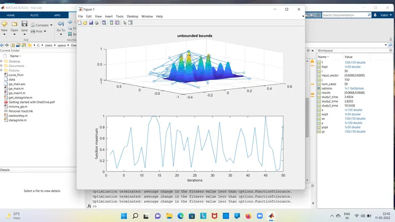
If the study1 is plots of optimum solution of unbounded bounds in the ga,
subplot command is used for multiple plots in plot.
study timer is used commands is tic and toc ,optimum solutions to study timer ,required time taken.
plot3 command is used for plot a surface of the plot.
title command is usd for title the study1,and also labelled to writen in axises.
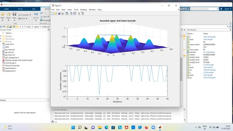
Study2-Bounded bounds is upper and lower bounds is the inputs,same code for study2 also,
some parameters are changes is upper and lower bounds.
The syntax of the study2 is x=ga(fun,nval,A,b,Aeq,beq,lb,ub)
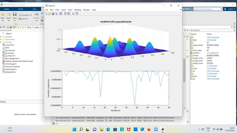
Study3-If the study3 is iterations / population size is increasing is 250 in study3.
optimoptions is used to increse the iteration/population size in study.
study3 is fit the global maxima .
syntax is x=ga(fun,nval,A,b,Aeq,beq,lb,ub,nonlcon,intcon,options)
% ERRORS IN CODE
% ERRORS OVERCOME IN CODE
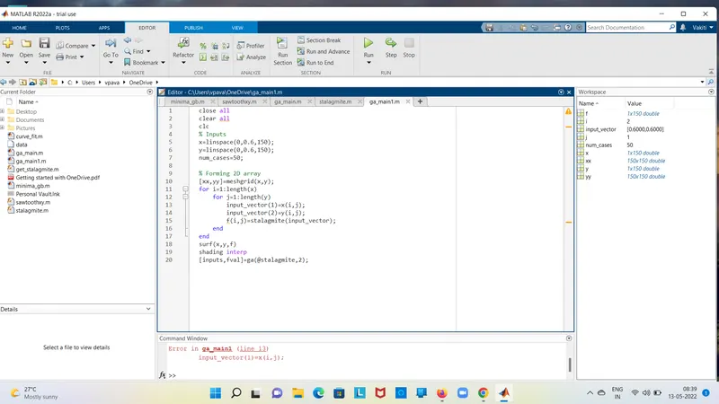
1 .input_vector(1)=x[i,j];
input_vector(2)=y[i,j];
The above line written id through an error.
Because Meshgrid in x and y is an 2D array.
input_vector(1)=xx[i,j];
input_vector(2)=yy[i,j];
The above line is to be correct.
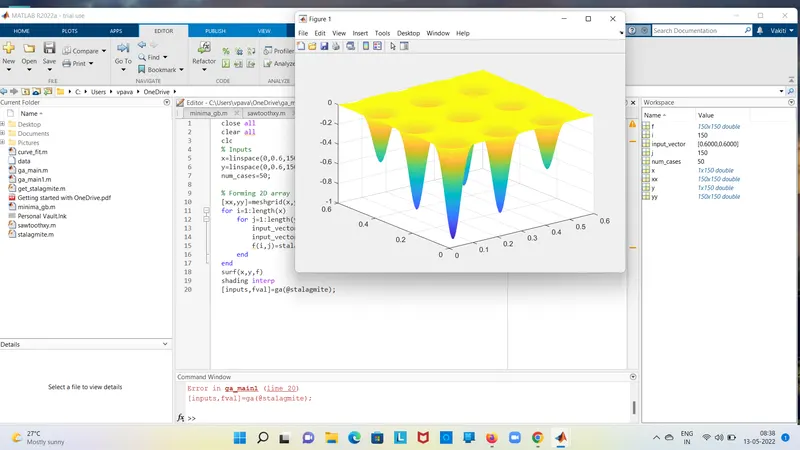
2. [inputs,fval]=ga(@stalagmite);
It will plot ,but through an error.
Because of 2 variables is x and y.
[inputs,fval]=ga(@stalagmite,2);
The above line to be written is correct.
close all
clear all
clc
% Inputs
x=linspace(0,0.6,150);
y=linspace(0,0.6,150);
num_cases=50;

% Forming 2D array
[xx,yy]=meshgrid(x,y);
for i=1:length(x)
    for j=1:length(y)
        input_vector(1)=xx(i,j);
        input_vector(2)=yy(i,j);
        f(i,j)=stalagmite(input_vector);
    end
end

% study1_ Statistical behavior of unbounded bounds
tic
for i=1:num_cases
    [results,fopt(i)]=ga(@stalagmite,2);
    xopt(i)=results(1);
    yopt(i)=results(2);
end
study1_time=toc;
figure(1)
subplot(2,1,1)
surf(x,y,-f)
shading interp
hold on
plot3(xopt,yopt,-fopt,'marker','o')
title('unbounded bounds')
subplot(2,1,2)
plot(-fopt)
xlabel('iterations')
ylabel('function maximum')

% Study2_statistical behavior of bounded upper and lower bounds
tic
for i=1:num_cases
    [results,fopt(i)]=ga(@stalagmite,2,[],[],[],[],[0;0],[0.6;0.6]);
    xopt(i)=results(1);
    yopt(i)=results(2);
end
study2_time=toc;
figure(2)
subplot(2,1,1)
surf(x,y,-f)
shading interp
hold on
plot3(xopt,yopt,-fopt,'marker','o')
title(' bounded upper and lower bounds')
subplot(2,1,2)
plot(-fopt)
xlabel('iterations')
ylabel('function maximum')
% Study3_Statistical behavior of GA increasing
options=optimoptions('ga');
options=optimoptions(options,'populationsize',250);
tic
for i=1:num_cases
    [results,fopt(i)]=ga(@stalagmite,2,[],[],[],[],[0;0],[0.6;0.6],[],[],options);
    xopt(i)=results(1);
    yopt(i)=results(2);
end

study3_time=toc;
figure(3)
subplot(2,1,1)
surf(x,y,-f)
shading interp
hold on
plot3(xopt,yopt,-fopt,'marker','o')
title(' modified with populationsize')
subplot(2,1,2)
plot(-fopt)
xlabel('iterations')
ylabel('function maximum')


% Stalagmite Function code
function [f]=stalagmite(input_vector)
x=input_vector(1);
y=input_vector(2);

f1x=(sin(5.1*pi*x+0.5)).^6;
f1y=(sin(5.1*pi*y+0.5)).^6;
f2x=exp((-4*log(2)*((x-0.0667).^2))/0.64);
f2y=exp((-4*log(2)*((y-0.0667).^2))/0.64);
f=-(f1x*f1y*f2x*f2y);
end
OUTPUT - MODIFIED POPULATION SIZE
OUTPUT-BOUNDED UPPER AND LOWER BOUNDS
OUTPUT-UNBOUNDED