Week 3 - Solving second order ODEs

% ORDINARY DIFFERENTIAL EQUATIONAL 2ND ORDER CODE EXPLAINATION FILE

% ODE 2ND ORDER SIMPLE PENDULUM WITH DAMPING

If an Ordinary Differential Equation 2nd Order ,to convert with 1st Order ODE,If the ODE to use pendulum moves , pendulum moves on Newton 2nd law , if the ball moves on with respect to time.

If the pendulum moves with time,velocity and theta (given theta based on angle to moves),If the function time pendulum moves.

If these vechile dynamics , suspenstion system of the vechile to pendulum moves like to see.

If the b is a damped,damping is a vibratory motion such as mechanical osscilations.

If g is a gravity of the bob ,gravity is a body to atract the towars the Earth.

m is a mass of the bob.

L is a length of the pendulum is quality in clock.

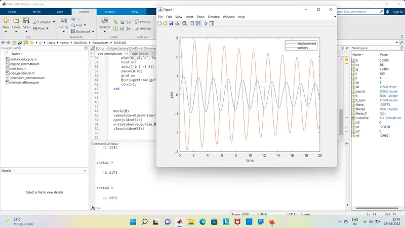
If the displacement is 0,velocity is from 3.

If the theta_0 values is taken from dispalcement and velocity.

t_span is a initial and final values of the time ,two-element vector.

If the 't' is a displacement values is 0.

If the "result" is a velocity values is 3.

ode45 is built in function,to solve ODE order ,ode_func is a function to call values is (t,theta,b,g,l,m).

If the plot 1 is plott the velocity.

If the plot 2 is plott the displacement.

If the "for " loop is use requiry number of times theta values ,If the "for" loop is a calls a know times.

If the "for" loop is use pendulum motion requiry times.

If the plot 1 is the wall sturdy, to plott the given 'color', and 'linewidth'.

If the plot 1 is the massless rod is to create ,it's 'color', and 'linewidth' is to requiry be given,by user.

If plot 2 is the BOB is creates ,if sphere size is given user to command "markers",'color' is to be given by user.

Animation is created by "COMMANDS " of the Movie.

% ERROR FACE IN CODE .

% ERROR IS OVERCOME IN CODE.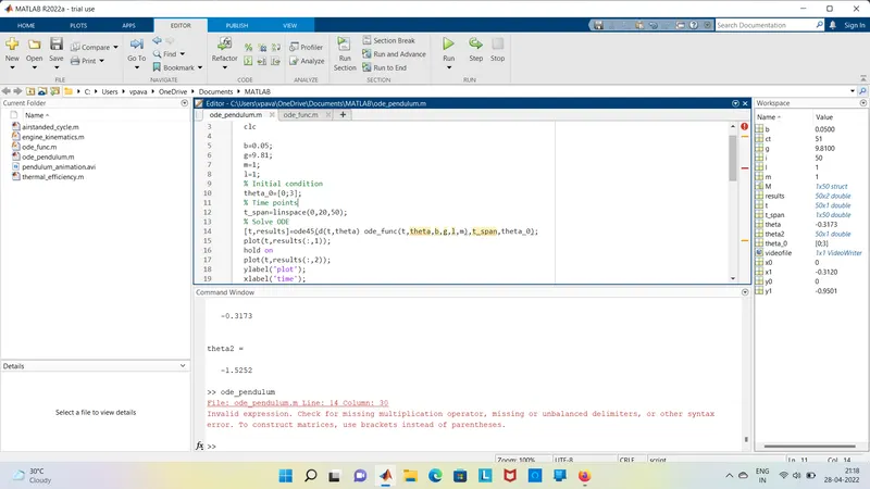

1 [t,results]=ode45(d(t,theta) ode_func(t,theta,b,g,l,m),t_span,theta_0);

It will through an error ,the above line written,because of 'd' is a variable.

[t,results]=ode45(@(t,theta) ode_func(t,theta,b,g,l,m),t_span,theta_0);

The above line is given correct one ,Because of '@' in a function calling superclass methods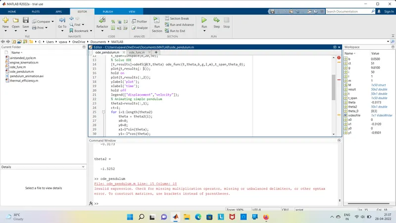

2 plot(t,results(: 1));

The above shows an Error , it an expression error,operator error,it will not run code.

plot(t,results(:,1));

The above one overcome the error,if the "comma" is repressents an expression,it run code.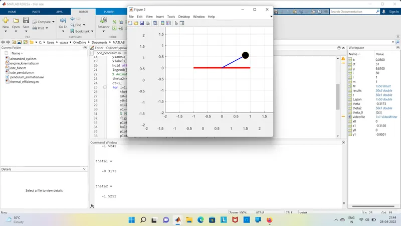

3 % Animating simple pendulum

theta2=results(:,2);

The above shows runs code and plot ,but pendulum animation is not proper we required, theta is angles changes with pendulum osscilations.

theta2=results(:,1);

The above one overcome proper we required pendulum moves.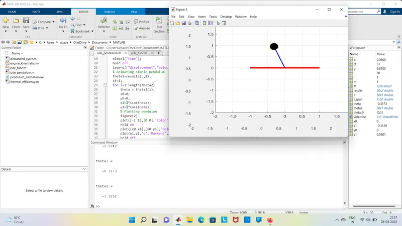

4 y1=l*cos(theta);

It will runs the code but pendulum osscilations to be in upwards on wall sturdy.

y1=-l*cos(theta);

The above line gives a pendulum required osscilations.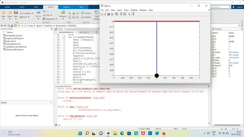

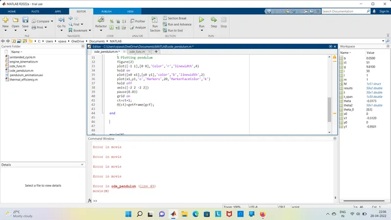
5 axis([2 2 2 2])

The above line will not given proper pendulum and through error, Because second value and first

value are equal.

axis([-2 2 -2 2])

It will gives a proper pendulum , Because second value is greaterthan the first value.

6 ct=ct+1;

M(ct)=getframe(gcf);

It will code and animation,but movie is not created , it is an uninitiallize movie.

M(ct)=getframe(gcf);

ct=ct+1;

The above one shows created a movie ,because of ct=ct+1 before M(ct)=getframe(gcf),Initiallize

the movie frame .

7 writeVideo(videofile)

It will through an error,because it is "not enough arguments".

writeVideo(videofile,M)

It will create a movie ,"movie(M)" if the "M" is the creates movie .

% ODE45

[t,results]=ode45(@(t,theta) ode_func(t,theta,b,g,l,m),t_span,theta_0))

ode45 is the built-in functions,only two arguments [t,results].

If the ode45 is a accurate method.

compares methods four to five orders estimate error and determine step size.

If the ode45 is only solve 1st order ode,remaining higher orders is converted into a 1st order ode.

close all
clear all
clc

b=0.05;
g=9.81;
m=1;
l=1;
% Initial condition
theta_0=[0;3];
% Time points
t_span=linspace(0,20,500);
% Solve ODE
[t,results]=ode45(@(t,theta) ode_func(t,theta,b,g,l,m),t_span,theta_0);

%plotting
plot(t,results(:,1));
hold on
plot(t,results(:,2));
ylabel('plot');
xlabel('time');
hold off
legend(["displacement","velocity"]);
% Animating simple pendulum
theta2=results(:,1);
ct=1;
for i=1:length(theta2)
    theta = theta2(i);
    x0=0;
    y0=0;
    x1=l*sin(theta);
    y1=-l*cos(theta);
    % Plotting pendulum
    figure(2)
    plot([-1 1],[0 0],'Color','r','linewidth',4)
    hold on
    plot([x0 x1],[y0 y1],'color','b','linewidth',2)
    plot(x1,y1,'o','Markers',20,'MarkerFaceColor','k')
    hold off
    axis([-2 2 -2 2])
    pause(0.03)
    grid on
    M(ct)=getframe(gcf);
    ct=ct+1;
end


% Animation movie
movie(M)
videofile=VideoWriter('pendulum_animation.avi','uncompressed AVI');
open(videofile)
writeVideo(videofile,M)
close(videofile)