Week 4.1 - Genetic Algorithm
Aim:-
- Write a code in MATLAB to optimise the stalagmite function and find the global maxima of the function
Introduction:-
Genetic Algorithm (GA) is a search-based optimization technique based on the principles of Genetics and Natural Selection. It is frequently used to find optimal or near-optimal solutions to difficult problems which otherwise would take a lifetime to solve. It is frequently used to solve optimization problems, in research, and in machine learning.
Theory:-
What is Optimization?
- Optimization refers to finding the values of inputs in such a way that we get the “best” output values. The definition of “best” varies from problem to problem, but in mathematical terms, it refers to maximizing or minimizing one or more objective functions, by varying the input parameters.
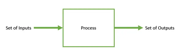
- The set of all possible solutions or values which the inputs can take make up the search space. In this search space, lies a point or a set of points which gives the optimal solution. The aim of optimization is to find that point or set of points in the search space.
What is stalagmite function?
- A stalagmite is a type of speleothem that rises from the floor of a limestone cave due to the dripping of mineralized solutions and the deposition of calcium carbonate.
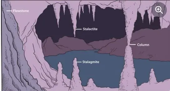
- In MATLAB a stalagmite function generally refers to the function with which we are generating values over a stalagmite kind of surface for finding out the local and global maxima and minima of that particular given function.
Defination of Genetic algorithm :-
- A genetic algorithm (GA) is a metaheuristic inspired by the process of natural selection that belongs to the larger class of evolutionary algorithms (EA). Genetic algorithms are commonly used to generate high-quality solutions to optimization and search problems by relying on biologically inspired operators such as mutation, crossover and selection.
- The genetic algorithm is a technique for solving both constrained and unconstrained optimization problems that are based on natural selection, the process that drives biological evolution. The genetic algorithm constantly modifies the population size of individual solutions.
Phases or Process of Genetic algorithm(GA):-
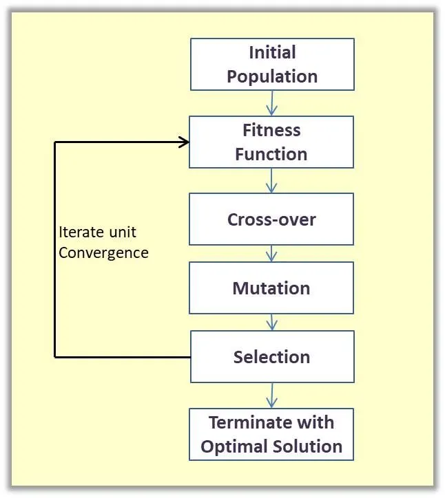
1.Initialization of Population (Coding) :-
- The code generates its random population of defined size and from that population the code evaluates the fitness of the members of the population according to which it forms new population based on no. of iterations performed.
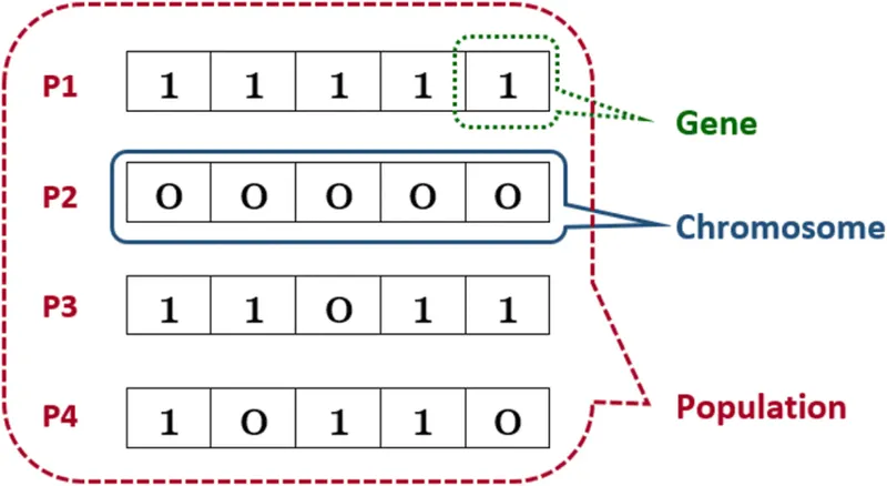
2.Fitness Function :-
- It is that function which we have to optimize and its optimization is done with the help of number of generations which have been formed by the code accordance with the fitness value of each member generated, these fitness values are used for the reproduction of the children.
- It also defined as a function which takes a candidate solution to the problem as input and produces as output how “fit” our ,how “good” the solution is with respect to the problem in consideration.
-
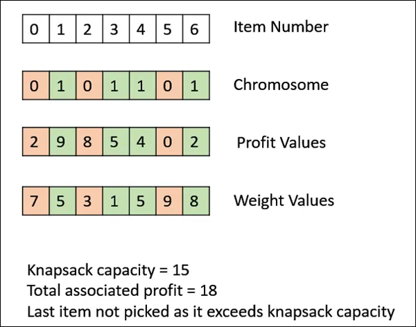
The following image shows the fitness calculation for a solution of the 0/1 Knapsack. It is a simple fitness function which just sums the profit values of the items being picked (which have a 1), scanning the elements from left to right till the knapsack is full.
3.Selection :-
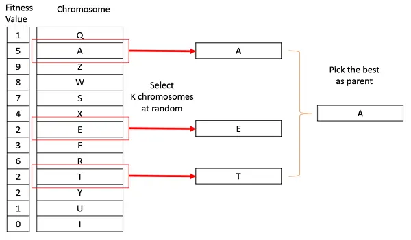
- The idea of the selection phase is to select the fittest individuals and let them pass their genes to the next generation. The main goal of this phase is to find the region where the chances of getting the best solution are more.
- Inspiration for this is from the survival of the fittest.
- It should be a balance between exploration and exploitation of search space.
- GA tries to move the genotype to higher fitness in the search space.
- Too strong fitness selection bias can lead to sub-optimal solutions.
- Too little fitness bias selection results in unfocused search.
4.Reproduction :-
- Generation of offspring happen in 2 way:
- Crossover
- Mutation
4(a) Crossover :-
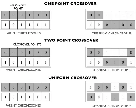
Crossover is the most significant stage in the genetic algorithm. During crossover, a random point is selected while mating a pair of parents to generate offspring.
There are 3 major types of crossover.
Single Point Crossover:
A point on both parents’ chromosomes is picked randomly, and designated a ‘crossover point’.
Two-Point Crossover: Two crossover points are picked randomly from the parent chromosomes.
Unifofm Crossover: In a uniform crossover, typically, each bit is chosen from either parent with equal probability.
4(b) Mutation :-
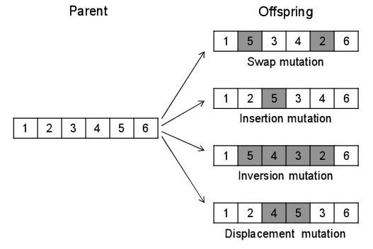
In a few new offspring formed, some of their genes can be subjected to a mutation with a low random probability. This indicates that some of the bits in the bit chromosome can be flipped. Mutation happens to take care of diversity among the population and stop premature convergence.
Syntax for genetic algorithm :-
- x = ga(fun,nvars)
- x = ga(fun,nvars,A,b)
- x = ga(fun,nvars,A,b,Aeq,beq)
- x = ga(fun,nvars,A,b,Aeq,beq,lb,ub)
- x = ga(fun,nvars,A,b,Aeq,beq,lb,ub,nonlcon)
- x = ga(fun,nvars,A,b,Aeq,beq,lb,ub,nonlcon,options)
- x = ga(fun,nvars,A,b,[],[],lb,ub,nonlcon,IntCon)
- x = ga(fun,nvars,A,b,[],[],lb,ub,nonlcon,IntCon,options)
- x = ga(problem)
- [x,fval] = ga(___)
- [x,fval,exitflag,output] = ga(___)
- [x,fval,exitflag,output,population,scores] = ga(___)
Description :-
x = ga(fun,nvars)finds a local unconstrained minimum,x, to the objective function,fun.nvarsis the dimension (number of design variables) offun.x = ga(fun,nvars,A,b)finds a local minimumxtofun, subject to the linear inequalitiesA*x≤b.gaevaluates the matrix productA*xas ifxis transposed (A*x').x = ga(fun,nvars,A,b,Aeq,beq)finds a local minimumxtofun, subject to the linear equalitiesAeq*x=beqandA*x≤b. (SetA=[]andb=[]if no linear inequalities exist.)gaevaluates the matrix productAeq*xas ifxis transposed (Aeq*x').x = ga(fun,nvars,A,b,Aeq,beq,lb,ub)defines a set of lower and upper bounds on the design variables,x, so that a solution is found in the rangelb≤x≤ub. (SetAeq=[]andbeq=[]if no linear equalities exist.)x = ga(fun,nvars,A,b,Aeq,beq,lb,ub,nonlcon)subjects the minimization to the constraints defined innonlcon. The functionnonlconacceptsxand returns vectorsCandCeq, representing the nonlinear inequalities and equalities respectively.gaminimizes thefunsuch thatC(x)≤0andCeq(x) = 0. (Setlb=[]andub=[]if no bounds exist.)x = ga(fun,nvars,A,b,Aeq,beq,lb,ub,nonlcon,options)minimizes with the default optimization parameters replaced by values inoptions. (Setnonlcon=[]if no nonlinear constraints exist.) Createoptionsusingoptimoptions.x = ga(fun,nvars,A,b,[],[],lb,ub,nonlcon,IntCon)orx = ga(fun,nvars,A,b,[],[],lb,ub,nonlcon,IntCon,options)requires that the variables listed inIntContake integer values.x = ga(problem)finds the minimum forproblem, a structure described inproblem.[x,fval] = ga(___), for any previous input arguments, also returnsfval, the value of the fitness function atx.[x,fval,exitflag,output] = ga(___)also returnsexitflag, an integer identifying the reason the algorithm terminated, andoutput, a structure that contains output from each generation and other information about the performance of the algorithm.[x,fval,exitflag,output,population,scores] = ga(___)also returns a matrixpopulation, whose rows are the final population, and a vectorscores, the scores of the final population.
Code for stalagmite function :-
function F=stalagmite(input_vector)
x=input_vector(1)
y=inpt_vector(2)
f1_x = (sin((5.1*pi*x)+.5))^6;
f1_y = (sin((5.1*pi*y)+.5))^6;
f2_x = exp((-4*log(2)*(x-0.0667)^2)/0.64);
f2_y = exp((-4*log(2)*(y-0.667)^2)/0.64);
F =-( f1_x*f1_y*f2_x*f2_y)
Explanation of the above function :-
The above code is used to make stalagmite function which will help in plot the graph in main command.
`f(x,y)=f_1,x*f_2,x*f_1,y*f_2,y`
`f_1,x=[sin(5.1pix+0.5)]^6`
`f_2,y=[sin(5.1piy+0.5)]^6`
`f_2,x=exp[-4ln(2)(x-0.0667)^2/.64]`
`f_2,y=exp[-4ln(2)(y-0.0667)^2/.64]`
- While using the function at the end as we are using the -ve sign so that the plot will be reversed as we have to find the maxima of the given function using ga.
Code for optimise the stalagmite function and find the global maxima of the function:-
Explanation of the above code :-
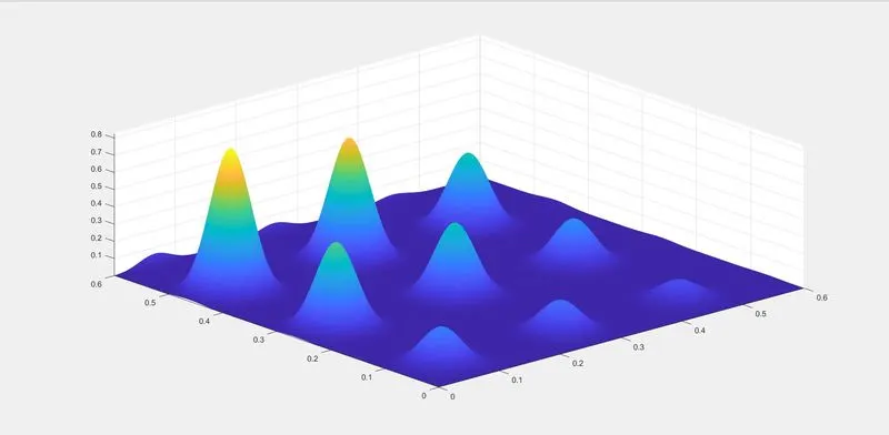
- Firstly we create the meshgrid(2d vector) from the 1d vector(x and y) which acting as search space for the stalagmite function.
- Now calculating the values of fitness function at each point of the mesh grid formed.
- Here we used "surfc" command for generating contour of the stalagmite function.
- While using surfc applying the -ve sign to the function will generate the surface upside down which will be quite good to get the maxima of the function, as it will provide positive value for the maxima using the -ve sign.
- shading interp command is used to remove the line from the contour surface.
Code for the plot surface of stalagmite function :-
close all
clear all
clc
% providing search space for the function
x=linspace(0,.6,150);
y=linspace(0,.6,150);
n=50; %Number of iteration for which the function will evalute the fittnes
[xx yy]= meshgrid(x,y);
%creating surface plot of the the stalagmite function
for i=1:length(xx);
    for j=1:length(yy);

    input_vector(1)=xx(i,j);
    input_vector(2)=yy(i,j);
     F(i,j) = stalagmite(input_vector);%the value of argument is defined in search space
end
end

surfc(xx,yy,-F)%creating surface plot
shading interp
This is the plot of the above code:-
Case1 :- Study statistical behaviour without boundation of the stalagmite function :-
- Here We used 'tic' and 'toc' command for calculating how much time taken to slove the genetic algorithm.
- Then plotting it into the surf command and also providing the optimum values of the function that how it is varying.
- we used negative sign because we want to calculate global maxima.
- For loop is used to run the ga 50 times.
- Through ga we calling stalagmite function and give the no. of variable that is 2.
- Though the ga we will get 2 outputs these are
- xout(i)=input_vector(1)
- yout(i)=input_vector(2)
- And plot the graph using plot3 command.
plot3( plots coordinates in 3-D space.X,Y,Z)
-
To plot a set of coordinates connected by line segments, specify
X,Y, andZas vectors of the same length. -
To plot multiple sets of coordinates on the same set of axes, specify at least one of
X,Y, orZas a matrix and the others as vectors.
Code :-
This is the plot of above code :-
close all
clear all
clc
% providing search space for the function
x=linspace(0,.6,150);
y=linspace(0,.6,150);
n=50; %Number of iteration for which the function will evalute the fittnes
[xx yy]= meshgrid(x,y);
%creating surface plot of the the stalagmite function
for i=1:length(xx);
    for j=1:length(yy);

    input_vector(1)=xx(i,j);
    input_vector(2)=yy(i,j);
     F(i,j) = stalagmite(input_vector);%the value of argument is defined in search space
end
end

surfc(xx,yy,-F)%creating surface plot
shading interp

% case1:-study statistical behaviour without boundation
tic
for i=1:n
    [input_vector,Fopt(i)]=ga(@stalagmite,2);
        xout(i)=input_vector(1);
        yout(i)=input_vector(2);
end
case1_time=toc;

figure(1)
subplot(2,1,1);
surfc(xx,yy,-F)%create the surface of stalagmite function
shading interp % Remove the line, which plot on the surface because of meshgrid
xlabel('x-axis');
ylabel('y-axis');
hold on
plot3(xout,yout,-Fopt,'marker','o','markersize',5,'markerfacecolor','r')
title('Unbounded Inputs');
subplot(2,1,2);
plot(-Fopt)
xlabel('Iteration');
ylabel('Function maximum');

tic
%case2:-statical behaviour with upper and lower boundries

for j=1:n
    [inputs,Fopt(j)]=ga(@stalagmite,2,[],[],[],[],[0;0],[0.6;0.6]);
    xout(j)=inputs(1);
    yout(j)=inputs(2);
end
case2_time=abs(toc);
figure(2)
subplot(2,1,1);
surfc(xx,yy,-F);
xlabel('X-axis');
ylabel('Y-axis');
shading interp
hold on
plot3(xout,yout,-Fopt,'marker','o','markersize',5,'markerfacecolor','r');
title('Bounded inputs');
subplot(2,1,2);
plot(-Fopt);
xlabel('Iteration');
ylabel('Function maximum');

tic
%case3:- study statical behaviour of a bounded inputs with increase in population size
options=optimoptions('ga');
options=optimoptions(options,'populationsize',300)

for k=1:n
    [inputs,Fopt(k)]=ga(@stalagmite,2,[],[],[],[],[0;0],[0.6;0.6],[],[],options);
    xout(k)=inputs(1);
    yout(k)=inputs(2);
end
case3_time=toc;

figure(3)
subplot(2,1,1);
surfc(xx,yy,-F);
shading interp
hold on
plot3(xout,yout,-Fopt,'marker','o','markersize',5,'markerfacecolor','r');
title('Bounded with population size increase');
subplot(2,1,2);
plot(-Fopt);
xlabel('Iteration');
ylabel('Function maximum');
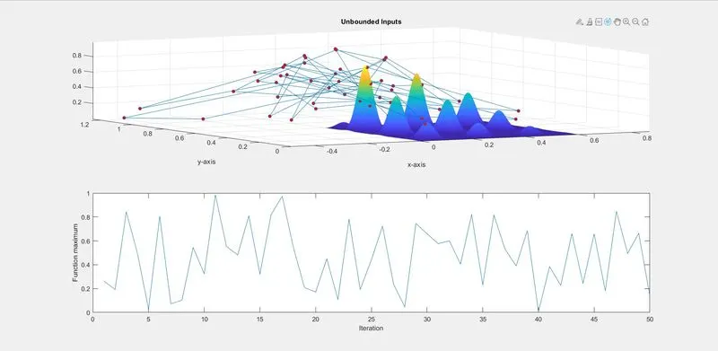
- time taken for study ga is 94.47259 sec
- we can improve the plot by giving the limit in the x and y.
Case-2 :- optimise the stalagmite function with boundation :-
- The difference over here is in providing the upper and the lower limit in the ga so that the search space is reduced with the upper and lower boundary and then plotting it as similar to the above study.
- we give the boundation from 0 to 0.6.
Code :-
tic
%case2:-statical behaviour with upper and lower boundries

for j=1:n
    [inputs,Fopt(j)]=ga(@stalagmite,2,[],[],[],[],[0;0],[0.6;0.6]);
    xout(j)=inputs(1);
    yout(j)=inputs(2);
end
case2_time=abs(toc);
figure(2)
subplot(2,1,1);
surfc(xx,yy,-F);
xlabel('X-axis');
ylabel('Y-axis');
shading interp
hold on
plot3(xout,yout,-Fopt,'marker','o','markersize',5,'markerfacecolor','r');
title('Bounded inputs');
subplot(2,1,2);
plot(-Fopt);
xlabel('Iteration');
ylabel('Function maximum');
This is the plot of above code :-
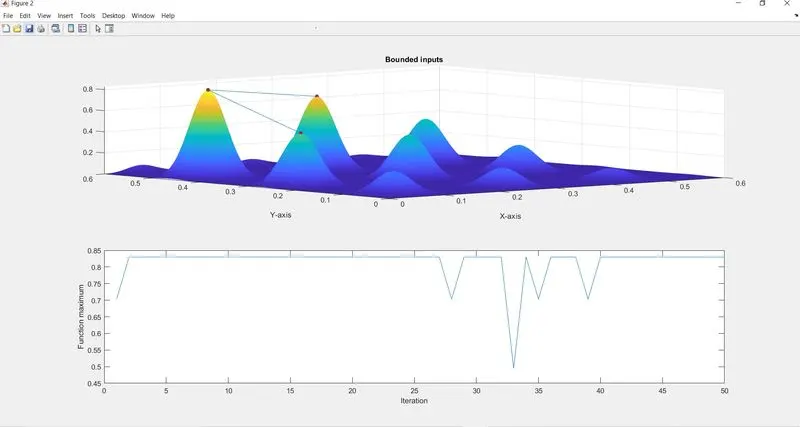
- The time taken for the study ga is 93.79339
- further we can improve the grap by increasing the plopulation size.
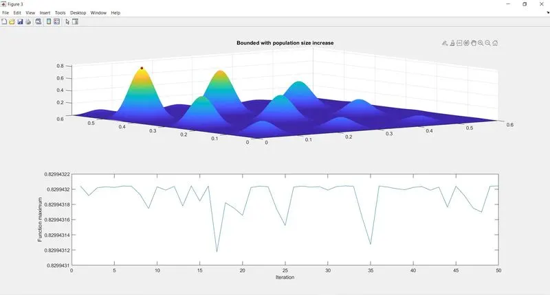
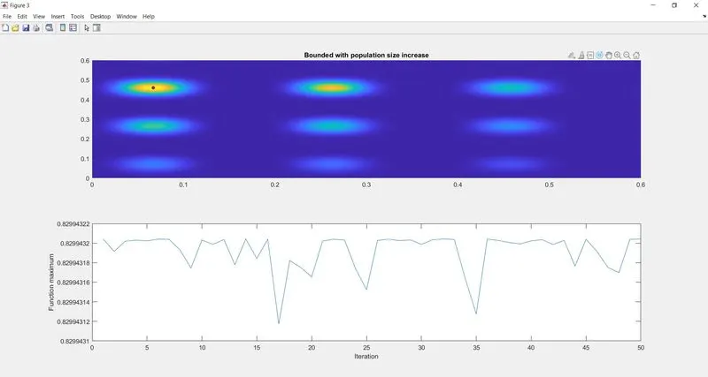
Case3 :- study statistical behaviour with bounded inputs and increasing population size
-
In this study using the ‘optimoptions’ command to increase the size of population.
- we incerease the population size to 300.
-
The benefit of that will be it will be working on the large set of numbers and which will be led to increase the possibilities of finding the better fitness of the function.
-
The drawback is that the time for evaluation will increase.
Code :-
tic
%case3:- study statical behaviour of a bounded inputs with increase in population size
options=optimoptions('ga');
options=optimoptions(options,'populationsize',300)

for k=1:n
    [inputs,Fopt(k)]=ga(@stalagmite,2,[],[],[],[],[0;0],[0.6;0.6],[],[],options);
    xout(k)=inputs(1);
    yout(k)=inputs(2);
end
case3_time=toc;

figure(3)
subplot(2,1,1);
surfc(xx,yy,-F);
shading interp
hold on
plot3(xout,yout,-Fopt,'marker','o','markersize',5,'markerfacecolor','r');
title('Bounded with population size increase');
subplot(2,1,2);
plot(-Fopt);
xlabel('Iteration');
ylabel('Function maximum');- time taken to study the ga is 663.2710
This is the plot of above code :-
Conclusion :-
- Here we seen that we can improve the the optimization through changing the condition for the optimization such as :-
Give the boundary condition for the optimization.
increase in population size.
- But while increasing the condition for the optimization though ga the time required for the optimization also increased.
- So we can get a optimum result through ga but there it take a littile more time to evaluate the result.