Project 2 - Rankine cycle Simulator

Aim :-

write a MATLAB code to creat a Rankine cycle

Govering Equation :-

work output(`W_o`)=`h_1`-`h_2`

Work input(`W_i`)=`h_4`-`h_3`

Net work output=`W_o`-`W_i`

Backwork Ratio= `W_i`/`W_o`

Here h=Specific enthalpy

Objective :-

• Creat a Rankine cycle Simulator
• Calculate the State point of the Rankine cycle
• Plot the corresponding temperature vs specific entropy and specific enthalpy vs specific entropy Diagram.
• Also Calculate Backwork Ratio and Net work output

Theory :-

• The Rankine cycle, also called the Rankine vapor cycle, is a thermodynamic cycle that converts heat into mechanical energy. The Rankine cycle is name after William Johnson Macquorn Rankine, a 19th century Scottish engineer and physicist known for his research in the thermodynamic properties of steam.

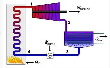
• The Rankine cycle makes practical use of the increase in pressure that occurs when a condensed fluid is forced to evaporate within a contained vessel. The cycle begins when a fluid, such as water, is compressed and put under high pressure. When the liquid is heated, the compressed fluid becomes a vapour that can be used to generate mechanical energy. When the heat is reduced, the vapour cools and condenses back to liquid form. The cycle then begins again.

Process in Rankine cycle :-

1-2 :- Internal Reversible Adiabatic expantion process (Turbine)

• In this process the saturated vapour enters into the turbine and expand adiabatically to wet vapour so that the turbine shaft rotate and the shaft is connected to a alternator to get the electricity.

2-3 :- Internal Reversible Isobaric Heat Rejection process(condenser)

• In this process the wet vapour which is coming from the turbine is condenced to the saturated liquid inside the condenser.

3-4 :- Internal Reversible Adiabatic compression process (Pump)

• In this process the saturated liquid is compressed adiabatically through the pump until it reaches to the boiler pressure.

4-1 :- Internal Reversible Isobsric Heat Addition process (Boiler)

• In this process the sub cooled liquid is compressed in a boiler to saturated vapour.

Main code :-

clear all
close all
clc
% the print description

fprintf('                        RANKINE CYCLE\n')
fprintf('1-2 Iinternally Reversible Adiabatic expansion in the turbine\n')
fprintf('2-3 Internally Reversible isobaric Heat rejection by the condenser\n')
fprintf('3-4 Internally Reversible Adiabatic compression by pump\n')
fprintf('4-1 Internally Reversible Isobaric Heat addition the boiler\n')

%Input all the required variable
p1=input('Enter the inlet pressure of the Turbine(in bar):');
T1=input('Enter the inlet tempersture of Turbine(in Degree celcius):');
p2=input('Enter the condenser pressure or turbine outlet pressure(in bar):');

%calculate all state value
%state1 all the value
h1=XSteam('h_pt',p1,T1);
s1=XSteam('s_pt',p1,T1);
%state 2 all the values
s2=s1;
hf2=XSteam('hL_p',p2);
hg2=XSteam('hV_p',p2);
sf2=XSteam('sL_p',p2);
sg2=XSteam('sV_p',p2); %x=(s2-sf2)/(sg2-sf2)
x2=(s2-sf2)/(sg2-sf2);
h2=hf2+[x2*(hg2-hf2)];  %hf2+(x(hg2-hf2)
T2=XSteam('T_hs',h2,s2);
%state 3 all the values
T3=T2;
p3=p2;
s3=XSteam('sL_p',p3);
h3=XSteam('hL_T',T3);
v3=XSteam('vL_T',p2);
% state point 4 all value 
p4=p1;
s4=s3;
Cp4=XSteam('Cp_ps',p4,s4);
Cv4=XSteam('Cv_ps',p4,s4);
gamma=Cp4/Cv4;
r=(gamma-1)/gamma;
T4=T3*(p4/p3)^r;
% calculate other variable
%work input in pump
Wp=v3*(p1-p2)*100;
% workdone by turbine
Wt=h1-h2;
%enthalpy at boiler input
h4=Wp+h3;
%Net Workdone 
W_net=Wt-Wp;
%Heat supplied to boiler
Qs=h1-h4;
%thermal efficiency 
N_per=(W_net/Qs)*100;
%back work ratio 
BWR=(Wp)/(Wt);
%specific steam consumption
SSC=3600/(W_net);
%State 5 and state 6 all values
T5=XSteam('TSat_p',p1);
T6=T5;
s5=XSteam('SL_P',p1);
s6=XSteam('sV_P',p1);
h5=XSteam('hL_P',p1);
h6=XSteam('hV_P',p1);

% Print all the values to show
fprintf('\n-------------------Result---------------------\n')
fprintf('At the state point 1 :\nP1 is : %4.2f Bar\nT1 is : %4.2f Degree celcius\nh1 is : %4.2f Kj/kg\ns1 is : %4.2f kj/kg-k\n\n',p1,T1,h1,s1)
fprintf('At the state point 2 :\nP2 is : %4.2f Bar\nT2 is : %4.2f Degree celcius\nX2 is : %4.2f \nh2 is : %4.2f Kj/kg\ns2 is : %4.2f kj/kg-k\n\n',p2,T2,x2,h2,s2)
fprintf('At the state point 3 :\nP3 is : %4.2f Bar\nT3 is : %4.2f Degree celcius\nh3 is : %4.2f Kj/kg\ns3 is : %4.2f kj/kg-k\n\n',p3,T3,h3,s3)
fprintf('At the state point 4 :\nP4 is : %4.2f Bar\nT4 is : %4.2f Degree celcius\nh4 is : %4.2f Kj/kg\ns4 is : %4.2f kj/kg-k\n\n',p4,T4,h4,s4);
fprintf('Workdone by turbine is : %4.2f Kj/kg \nWork input in pump is : %4.2f kj/kg\nNet workdone : %4.2f kj/kg\nThermal efficiency is : %4.2f percent\nBWR is : %4.2f\nSSC is : %4.2f kg/kwh ',Wt,Wp,W_net,N_per,BWR,SSC) 

% plot T-s diagram  
figure(1)
T_Rankine=linspace(T5,T1,5000);
for i=1:length(T_Rankine)
    s_Rankine(i) = XSteam('s_pT',p1,T_Rankine(i));
end
plot([s1 s2 s3 s4 s5 s6 s_Rankine],[T1 T2 T3 T4 T5 T6 T_Rankine],'linewidth',1.5)
hold on
T_curve = linspace(1,400,500);
for i=1:length(T_curve)
    s_l(i) = XSteam('sL_T',T_curve(i));
    s_V(i) = XSteam('sV_T',T_curve(i));
    h_L(i) = XSteam('hL_T',T_curve(i));
    h_V(i) = XSteam('hV_T',T_curve(i));
end
plot(s_l,T_curve,'color','g')
plot(s_V,T_curve,'color','g')
text(s1,T1,'1','Fontsize',15)
text(s2,T2,'2','Fontsize',15)
text(s3,T3,'3','Fontsize',15,'HorizontalAlignment','Right','VerticalAlignment','top')
text(s4,T4,'4','Fontsize',15,'HorizontalAlignment','Right','VerticalAlignment','bottom')
text(s5,T5,'5','Fontsize',15)
text(s6,T6,'6','Fontsize',15)
axis([0 10 0 600]);
title('Rankine cycle T-S Diagram');
xlabel('Entropy in Kj/Kg-K');
ylabel('Temperature in Degree Celcius');
%Now plot the H-s Diagram
figure(2)
plot([s1 s2 s3 s4 s1],[h1 h2 h3 h4 h1],'linewidth',1.5)
hold on
plot(s_V,h_V,'color','r')
plot(s_l,h_L,'color','r')

text(s1,h1,'1','Fontsize',15)
text(s2,h2,'2','Fontsize',15)
text(s3,h3,'3','Fontsize',15,'HorizontalAlignment','Right','VerticalAlignment','top')
text(s4,h4,'4','Fontsize',15,'HorizontalAlignment','Right','VerticalAlignment','bottom')
title('Rankine cycle H-S Diagram')
xlabel('Entropy Kj/Kg-K')
ylabel('Enthalpy kj/kg')

Explanation of the above code :-

• The above program is written for the make a Rankine cycle simulator .
• First we clear all the previous memory of the workspace through 'clear all' command.
• Here we take all the thermodynamic propoties like specific entropy ,specific enthalpy , specific Volume and Temperature value from a 'XSteam' Function Library.
• First we mention all the 4 process through the 'fprintf' Command.
• Then we need to input some specific data such as turbine input pressure and temperature and condensor pressure through 'input' command.
• Now we calculate all the state point of Rankine cycle thermodynamic propoties by using of XSteam function Library.
• Values of Entropy and Enthalpy a the function of pressure and temperature.
• h_pt,s_pt,sL_pt etc .. are the Default variable whose value is stored in XSteam Library.
• Pressure, Temperature, Enthalpy, Entropy for all the State Variables are Extracted as a function of the dependent variable from the XSteam File.
• The from state 2 to state 3 Low pressure saturated vapour is condenced to low pressure
  saturated liquid . hence Dryness fraction ,Enthalpy,Entropy for all the state variable are
  executed through XSteam function Library.
• For Calculating the pump work we need the Value of Specific Volume and Inlet and outlet pressure.
• Calculating the cp value used the command XSteam('cp_ps',p3,s3) here P3 and s3 is the depending argument.
• Now calculate the the workdone by the turbine and work input to the pump.
• Now to show all the state point thermodynamic value in command window we used the 'fprintf' command.
• For ploting we need two points these are point5 and point 6 to define the rankine cycle.
• Point 5 falls on the saturated liquid line and point 6 fall on the saturated vapour line for the given pressure.
• for Making saturated vapour and saturated liquid curve we need a set of temperature for the reference purpose.
• Now evalute the specific entropy and specific enthalpy on the saturated liquid and vapour line by using the Xsteam library and put the reference of given temperature range.
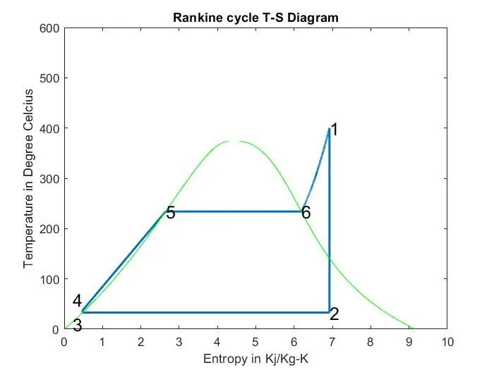
• Now plot the Rankine cycle T-s Diagram from above data.
• Mention all the state point through the "text" command.
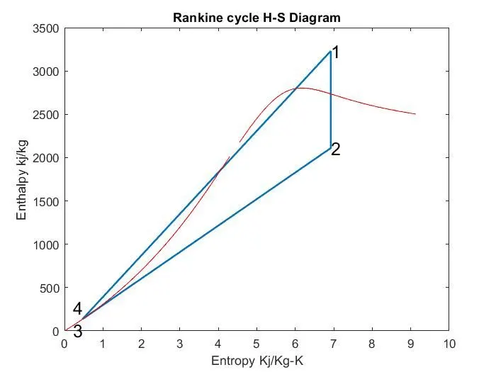
• Then plot the H-S Diagram of Rankine cycle.
• And also define all the state point.

This is the plot of Rankine T-S Diagram :-

This is the Rankine cycle H-S diagram :-

Command window :-

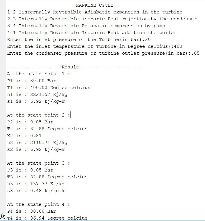
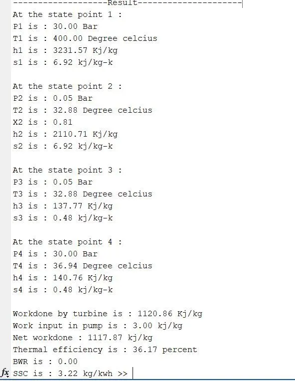
• Here Back work Ratio is Showing zero because the work input through the pump is very less as compare to the Turbine output value.

Conclusion :-

• In the above Rankine cycle ,the state 2 is fall in the Liquid and vapour region so it is not good for the turbine.
• The wet steam make dent on the turbine blade thats because the turbine is not use for long time period.
• So we need to further improve the Rankine cycle by using Regenerative and Reheating process.

Reference:-

• Wikipedia.com
• Mathworks.com