Week 3 - Solving second order ODEs

Aim :- The primary aim is to solve the given higer order differential equation that is `[d^2theta] /dt+b/m[d theta]/dt+g/lsin theta=0`and compute the displacement vector and velocity vector and secondary aim is to make a simulation of a motion of a simple pendulum`

Govering Equation :-

• we know that Newton second law of motion for the equation of a oscilating body describe in the manner that is :-
• `I [d^2 theta]/dt+b [d theta]/dt+theta=0`

Here 'I'=Moment of inertia

b=damping coefficient

`theta`=dispacement

t=time interval

OBJECTIVE :-

• The first objective is that to solve the given differential equation and calculate the displacement and velocity value for a given time interval of 0 to 20 sec and take the initial displacement is 0 and velocity is 3 rad/sec. and secondary objective is to make a simulation of a motion of simple pendulum by using above value
• g=gravity in `m/s^2` i.e 9.81
• l=length of the string i.e 1m
• m=mass of the ball i.e '1kg'
• b=damping coefficient i.e 0.05

The function code :-

function [dtheta_dt]=ode_func(t,theta,b,g,l,m)

theta1=theta(1);
theta2=theta(2);
dtheta1_dt=theta2;
dtheta2_dt=-b/m*theta2-(g/l)*sin(theta1);
dtheta_dt=[dtheta1_dt;dtheta2_dt];
end

Describe above function code :-

• Here we keep the function name is that ode_func.
• Here dtheta/dt is defined with independent variable 't' and dependent variable `theta`along with constant b,g,l,m.

The higher order defferential equation :-

`[d^2theta]/dt+b/m[d theta]/dt+g/lsintheta=0`

Let `theta=theta1`

`[d theta]/dt = [d theta_1]/dt = theta2` ----------------(1)`

`[d^2 theta]/dt = [d^2 theta_1]/dt = [d theta_2]/dt` --------(2)`

Now converting higer order to first order DE :-

`therefore [d^2 theta]/dt^2 + b/m[d theta]/dt + g/lsintheta =0`

`[d theta_2]/dt + b/m theta_2 + g/msintheta_1=0`

`[d theta_2]/dt=-b/m(theta2)-g/lsin(theta1)`

The first order DE vector value :-

`theta=[[theta1],[ theta2]]`

`d_theta/dt=[[[d theta_1]/[dt]] , [[d theta2]/[dt]]]`

Hence

`d/dt[[theta_1],[theta_2]]=[[theta_2],[-b/mtheta_2-g/lsintheta_1]]`

MAIN COMMAND CODE :-

clear all
close all
clc

%program for compute displacement and velocity vector create a pendulum motion animation

%input required variable
b=.05; % damping coefficient
g=9.81; %unit in m/s^2
l=1; %length in metre
m=1; %mass in kg

%initial condition
theta_0 = [0;3] %(initial angular displacement and angular velocity )
t_span=linspace(0,20,500); % how much time you want to observe

%solve code
[t,results]=ode45(@(t,theta)ode_func(t,theta,b,g,l,m),t_span,theta_0);

figure(1);
ct=1;
for i=1:length(t);
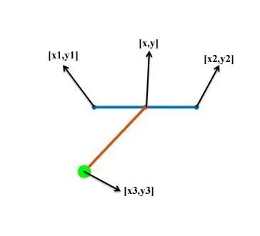
 x=0; % this is the pivot point of pendulum. & fixed end of the pendulum
 y=0; 
 
 x1=-.5;
 y1=0;
 
 x2=.5;
 y2=0;
 
 x3=l*sin(results(i,1));
 y3=-l*cos(results(i,1)); %this is the movable point of the pendulum
    
 plot([x1,x2],[y1,y2],[x,x3],[y,y3],'linewidth',2.1,'marker','o','markersize',2);
 hold on
 plot(x3,y3,'marker','o','markersize',10,'color','g','markerfacecolor','g')
 hold off
    axis([-2 2 -2 2]);
    M(ct)=getframe(gcf);
    title('pendulum motion');
    
    pause(0.05);
    ct=ct+1;
    
end 
       movie(M)
    videofile=VideoWriter('pendulum_motion.avi')
    open(videofile)
    writeVideo(videofile,M)
    close(videofile)
    
    figure(2)
    hold on
plot(t,results,'linewidth',2.1);
title('pendulum oscillation graph');
xlabel('time');
ylabel('displacement & velocity');
legend('angular displacement','angular velocity');

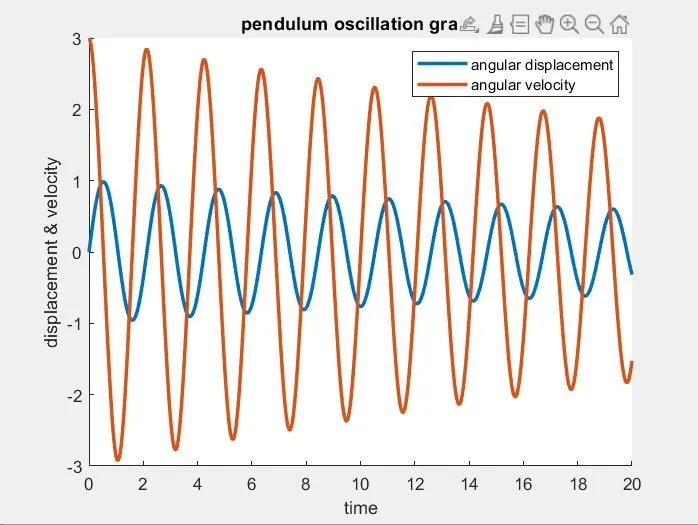
• The above command is written for calculate angular velocity and angular displacement of a pendulum for a given time interval
• And also make a animation video of simple pendulum and plot angular velocity and angular displacement curve with respect to time.
• Here ode45 is a function which is used to solve a higher order differential equation.
• It compares methods of orders four and five to estimate error and determine step size.
• These are the coordinates of pendulum :-

This is the plot of angular velocity and angular displacement with respect to time :-

This is the G-drive link of animation of pendulum:-

https://drive.google.com/file/d/1K6B0zB3Wo3tXVehy-HoyMpLGtI6CB8-W/view?usp=sharing

CONCLUSION:-

• Velocity and displacement vector is the function of time and theta.
• For the given time interval and Damping coefficient we cant't comes the pendulum in equilibrium state.
• Either increasing the time interval or Damping coefficient we can bring the pendulum in equilibrium condition.