Week 4.1 - Genetic Algorithm
Objective:
Write a code in Matlab to optimize the stalagmite function & find the global maxima of the function.
Definition of Genetic Algorithm:
Genetic algorithms (GA) are adaptive heuristic search algorithm that belongs to the larger part of evolutionary algorithms. Genetic algorithms are based on the ideas of naturals selection and genetics. These are intelligent exploitation of random search provided with historical data to direct the search into the region of better performance in solution space. They are commonly used to generate high-quality solutions for optimization problems and search problems.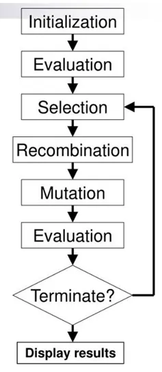
Genetic Algorithms are a class of search algorithms designed on the natural evolution process. GAs are based on the principles of survival of the fittest.
A Genetic Algorithm method inspired in the world of Biology, particularly, the Evolution Theory by Charles Darwin, is taken as the basis of its work. John Holland introduced the Genetic Algorithm in 1975. Genetic Algorithms are utilized to tackle optimization problems by copying the evolutionary behavior of species. From an initial random population of solutions, this population is advanced through selection, mutation, and crossover operators, inspired by natural evolution. By implementing the given set of operations, the population goes through an iterative procedure in which it reaches various states, and each one is called a generation. As a result of this procedure, the population is expected to reach a generation that contains a decent solution to the problem. In the Genetic Algorithm, the solution to the problem is coded as a string of bits or real numbers.
They have been shown in practice to be very efficient at functional optimization. It is used in searching for huge and sophisticated spaces. Genetic algorithms (GAs) are algorithms that are used for optimization and machine learning based on various features of biological evolution.
Phases of Genetic Algorithm:
- Initialization
- Evaluation-1
- Selection
- Recombination
- Mutation
- Evaluation-2
- Termination
Formula for Stalagmite function:
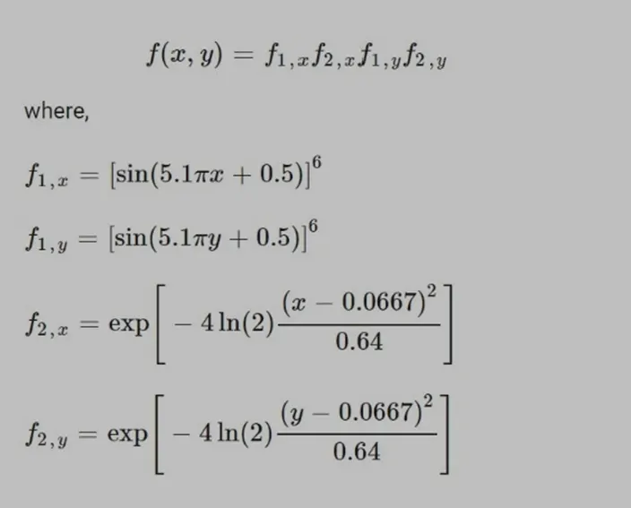
GA Syntax Description:
x= ga(fun,nvars,A,b,Aeq,beq,lb,ub,nonlcon,options)
Where,
x=local maxima point
fun=function to be called
nvars=no of variables
A,b,Aeq,Beq=inequalities in the function
lb=lower bound
ub=upper bound
nonlcon=two vectors representing inequalities & equalities
option=used to perform additional operation of optimoptions.
Code for Stalagmite function:
function [fxy]=stalagmite(input_vector)

x=input_vector(1);
y=input_vector(2);

f1x=(sin(5.1*pi.*x+0.5))^6;
f1y=(sin(5.1*pi.*y+0.5))^6;
f2x=exp(-4*log(2)*(x-0.0667)^2/0.64);
f2y=exp(-4*log(2)*(y-0.0667)^2/0.64);

fxy=-(f1x*f1y*f2x*f2y);
end
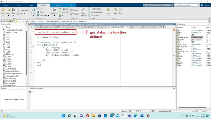
Code for get_stalagmite function:
function [f]=get_stalagmite1(x,y)

[xx,yy]=meshgrid(x,y);

% Evaluating the stalagmite function
for i=1:length(xx)
    for j=1:length(yy)
        input_vector(1)=xx(i,j);
        input_vector(2)=yy(i,j);
        f(i,j)=stalagmite(input_vector);

    end
end
end
Code for Study-1: statistical behavior without bounds
clear all
close all
clc

% Defining our search space
x=linspace(0,0.6,150);
y=linspace(0,0.6,150);
num_cases=60;
f=get_stalagmite1(x,y);

[xx,yy]=meshgrid(x,y);

% Evaluating the stalagmite function
for i=1:length(xx)
    for j=1:length(yy)
        input_vector(1)=xx(i,j);
        input_vector(2)=yy(i,j);
        f(i,j)=stalagmite(input_vector);

    end
end

% Study 1- statistical behaviour without bounds
tic
for i=1:num_cases
    [inputs,fopt(i)]=ga(@stalagmite,2);
    xopt(i)=inputs(1);
    yopt(i)=inputs(2);
    optf(i)=-fopt(i);


end
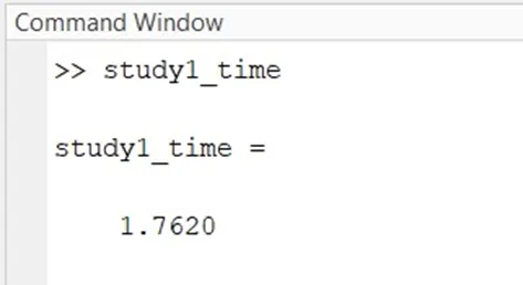
study1_time=toc;

figure(1)
subplot(2,1,1);
hold on
surfc(x,y,f);
shading interp
xlabel('X axis');
ylabel('Y axis');
zlabel('Z axis');
plot3(xopt,yopt,fopt,'marker','o','MarkerSize',5,'MarkerFaceColor','r')
title('Unbounded Inputs')
subplot(2,1,2)
plot(optf)
xlabel('No of Iteration');
ylabel('Function F maximum');
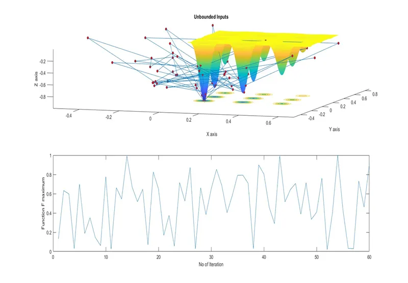
Result:
Code for Study-2: Statistical behavior with upper & lower bounds
clear all
close all
clc
% Defining our search space
x=linspace(0,0.6,150);
y=linspace(0,0.6,150);
f=get_stalagmite1(x,y);
[xx,yy]=meshgrid(x,y);

% Evaluating the stalagmite function
for i=1:length(xx)
    for j=1:length(yy)
        input_vector(1)=xx(i,j);
        input_vector(2)=yy(i,j);
        f(i,j)=stalagmite(input_vector);

    end
end

% Study 2-Statistical behaviour with upper & lower bounds
num_cases=100;

tic
for i=1:num_cases
   [inputs,fopt(i)]=ga(@stalagmite,2,[],[],[],[],[0;0],[1;1]);
   xopt(i)=inputs(1);
   yopt(i)=inputs(2);
   optf(i)=fopt(i);
end

study2_time=toc;

figure(3)
subplot(2,1,1)
hold on
surfc(x,y,f);
shading interp
xlabel('X axis');
ylabel('Y axis');
plot3(xopt,yopt,fopt,'marker','o','markersize',5,'markerfacecolor','k');
title(‘Bounded inputs’);
subplot(2,1,2);
plot(optf)
xlabel('No of Iteration');
ylabel('Function F Maximum');
max_value=fopt;
Result:
Code for Study-3: Statistical behavior of bounded inputs with an increase in population
clear all
close all
clc
% Defining our search space
x=linspace(0,0.6,150);
y=linspace(0,0.6,150);
f=get_stalagmite1(x,y);
[xx,yy]=meshgrid(x,y);

% Evaluating the stalagmite function
for i=1:length(xx)
    for j=1:length(yy)
        input_vector(1)=xx(i,j);
        input_vector(2)=yy(i,j);
        f(i,j)=stalagmite(input_vector);

    end
end

% Study 3- Statistical behavior of bounded inputs with increase in population
num_cases=150;
options=optimoptions('ga');
options=optimoptions(options,'populationsize',450);
tic
for i=1:num_cases
   [inputs,fopt(i)]=ga(@stalagmite,2,[],[],[],[],[0;0],[1;1],[],[],options);
   xopt(i)=inputs(1);
   yopt(i)=inputs(2);
   optf(i)=fopt(i);
end

study3_time=toc;

figure(3)
subplot(2,1,1)
hold on
surfc(x,y,f);
shading interp
xlabel('X axis');
ylabel('Y axis');
plot3(xopt,yopt,fopt,'marker','o','markersize',5,'markerfacecolor','k');
title('Bounded inputs with increase population size');
subplot(2,1,2);
plot(optf)
xlabel('No of Iteration');
ylabel('Function F Maximum');
max_value=fopt;
Result:
Stepwise procedure:
Step-1:
Click Window Start à Search ‘Matlab’ application. Once it appears on the window screen & Click the ‘Matlab’ icon.
Then Matlab application will be opened. Now first open the editor column & save the file name as ‘genetic_algorithm’.
Step-2:
Enter ‘clear all, close all, ctc commands.
The usages of the commands are shown below.
‘clear all’ command is used to clear all the data stored in the workspace.
‘close all’ command is used to cleart all graphs & plots.
‘clc’ is used to clear the command window.
Step-3:
In Study-1, the behaviour of algorithm is not defined with limits. Genetic algorithm doesn’t with a particular search space in this study-1 because of undefined boundaries.
Assign the parameters for study-1 to calculate the result of the statistical behaviour of the unbounded condition. Refer to the study-1 program code.
Step-4:
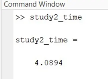
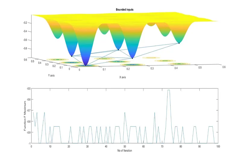
In study-2, the behaviour of the algorithm is defined with upper & lower limits in order to reduce the search space. Now, it is showing the result in 4 points.
Assign the parameters for study-1 to calculate the result of the statistical behaviour of the unbounded condition. Refer to the study-2 program code.
Step-5:
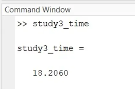
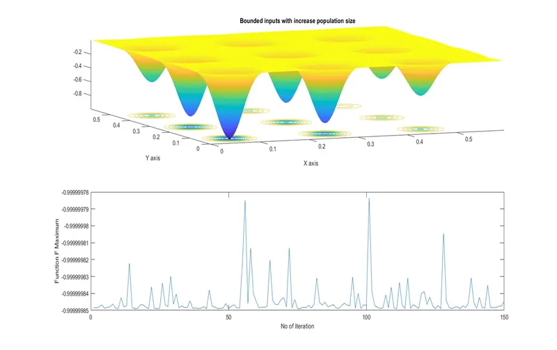
In study-3, the behaviour of the algorithm is defined with the bounding limits & also an increase in population size from 150 to 450. optimoptions() is used to change the ga variables to find the optimum solution.
Assign the parameters for study-1 to calculate the result of the statistical behaviour of the unbounded condition. Refer to the study-3 program code.
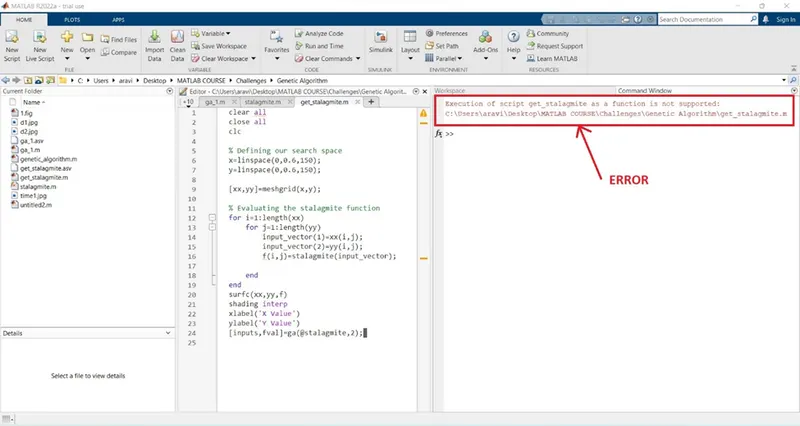
Errors faced during programming:
Steps taken to correct the error:
Conclusion:
While comparing all 3 studies, the below result is obtained.
- Study-3 has given optimum value but has taken long-running execution time.
- Study-1 has given an uncertain solution with a short period of execution time.
- Study-2 has given a moderate solution, which is between study-3 & study-1.
Reference Materials:
- https://www.educba.com/what-is-genetic-algorithm/
- https://www.geeksforgeeks.org/genetic-algorithms/
- https://matlab-code.org/genetic-algorithm-matlab/#:~:text=Genetic%20Algorithm%20consists%20a%20class%20of%20probabilistic%20optimization,a%20problem%2C%20each%20as%20fixed%20length%20character%20string.