Week 3 - Solving second order ODEs

Write a program to solve order differential equations in MATLAB & simulate the motion of the pendulum with damping.

Definition of ODE:

An ordinary differential equation contains the derivative of an unknown function. The ordinary differential equation is an equation having variables and a derivative of the dependent variable concerning the independent variable. The two types of ordinary differential equations are homogeneous and non-homogeneous differential equations.

The derivative of the dependent variable concerning only one independent variable is called the ordinary differential equation. A differential equation is an equation having variables and a derivative of the dependent variable concerning the independent variable. A differential equation contains at least one derivative of an unknown function, either an ordinary derivative or a partial derivative.

Applications of ODE:

Ordinary differential equations applications in real life include its use to calculate the movement or flow of electricity, study the to and fro motion of a pendulum, check the growth of diseases in graphical representation, mathematical models involving population growth, and radioactive decay studies.

Formula for solving the simple pendulum:

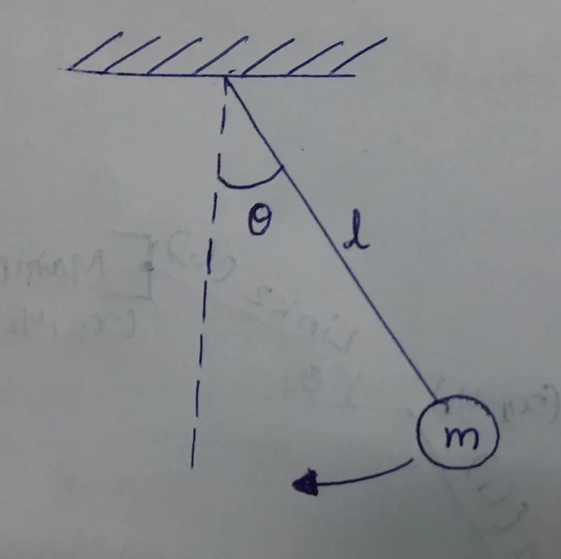
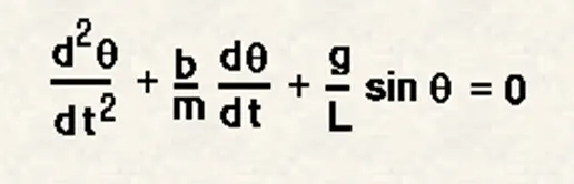
Where,

Θ=Angular Displacement

t=Tine (is seconds)

b= damping coefficient

m= Mass of Ball (in Kg)

l=length of string (in m)

g=gravity (in m/s^2)

MATLAB code:
clear all
close all
clc

%input values
%b=damping coefficient
%g=gravity in m/s^2
%l=length of the pendulum in m
%m=mass of the ball in kg

b=0.05;
g=9.81;
l=1;
m=1;

%inital condition
theta_0=[0,3];

% time points
t_span=linspace(0,20,500);

%solving ode

[t,results]=ode45(@(t,theta) ode(t,theta,b,g,l,m),t_span,theta_0);

%ploting the angular displacement & angular velocity 

figure(1)

plot (t,results(:,1),'linewidth',2)
hold on 
plot(t,results(:,2),'linewidth',2)
axis([0 20 -3 3])
xlabel('Time in seconds');
ylabel('Angular displacement & Angular velocity');
grid on
title('Damping Effect in Pendulum');
legend('Angular Displacement', 'Angular velocity')
pause(5);

% Simulation of the pendulum

ct=1;
for i=1:length(results(:,1))
    
x0=0;
y0=0;
x1=l*sin(results(i,1));
y1=-l*cos(results(i,1));

figure(2)
plot([x0,x1],[y0,y1],[-0.5 0.5],[0 0],'linewidth',3)
hold on
plot(x1,y1,'marker','o','markersize',25,'MarkerFaceColor','b')
axis([-2 2 -1.5 0.5])
grid on
title('Motion of the pendulum with damping')
pause(0.03)
M(ct)=getframe(gcf);
ct=ct+1;
hold off

end

% Movie file creation
movie(M)
videofile=VideoWriter('pendulum.avi','Uncompressed AVI');
open(videofile')
writeVideo(videofile,M)
close(videofile)


ODE function

function[dtheta_dt]=ode(t,theta,b,g,l,m)
theta1=theta(1);
theta2=theta(2);
dtheta1_dt=theta2;
dtheta2_dt=(-(b/m)*theta2-(g/l)*sin(theta1));
dtheta_dt=[dtheta1_dt; dtheta2_dt];
end

Stepwise Explanation of code:

Step-1

Click Windows Startà Search ‘Matlab’ application. Once it appears on the window screen & Clicks the ‘Matlab” icon.

Then Matlab application will be opened. Now open the editor column & save the file name as ‘second_ode’.

Add another tab in the editor window & save another file as ‘ode.m’.

Step-2

Enter ‘clear all, close all, ctc’ command.

The usages of the commands are shown below.

‘clear all’ command is used to clear all the data stored from the workspace.

‘close all’ command is used to close all graphs & plots

‘clc’ is used to clear the command window.

Step-3

Assign the input values for damping coefficient (b), gravity (unit-m/s^2)(g), length of the pendulum(l) (unit-meter), mass of the ball(m) (unit-kg).

b=0.05;

g=9.81;

l=1;

m=1;

Step-4

Assign values for angular displacement, angular velocity (rad/sec)

Angular displacement=0

Angular velocity=0

theta_0= [0,3];

Assign values for simulation time (0 to 20 seconds) with intermediate values 500.

t_span=linspace(0,20,500);

Step-5

Use ode45 inbuilt command to give the ode function in the main code.

[t,results]=ode45(@(t,theta) ode(t,theta,b,g,l,m),t_span,theta_0);

Step-6

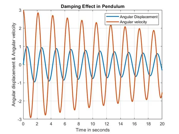
Type plot command to generate the graph between angular velocity & angular displacement against time.

plot (t,results(:,1),'linewidth',2)

hold on

plot(t,results(:,2),'linewidth',2)

assign values of the axis

axis([0 20 -3 3)

Step-7

Give X & Y axes with names as follows

xlabel('Time in seconds');

ylabel('Angular displacement & Angular velocity');

Type plot title & legend as follow,

title('Damping Effect in Pendulum');

legend('Angular Displacement', 'Angular velocity')

Step-8

Then assign the values to perform simulation of the pendulum

Assign the value of ct=1;

Start the for loop

ct=1;

for i=1:length(results(:,1))

x0=0;

y0=0;

x1=l*sin(results(i,1));

y1=-l*cos(results(i,1));

give x0, y0, x1, y1 values as the above.

Step-9

Type the below command to plot the pendulum with damper

figure(2)

plot([x0,x1],[y0,y1],[-0.5 0.5],[0 0],'linewidth',3)

hold on

plot(x1,y1,'marker','o','markersize',25,'MarkerFaceColor','b')

axis([-2 2 -1.5 0.5])

grid on

title('Motion of the pendulum with damping')

Step-10

Pause command is used to slow down the output video playback time.

pause(0.03)

Step-11

getframe command is used to get the individual frame from M variable.

M(ct)=getframe(gcf);

ct=ct+1;

hold off

Step-12

Type movie command to create movie file of output.

movie(M)

assign video file variable, for which movie file to be created.

Give the format of the movie file in VideoWriter function.

videofile=VideoWriter('pendulum.avi','Uncompressed AVI');

the below commands are used for opening, writing & closing the movie file.

open(videofile)

writeVideo(videofile,M)

close(videofile)

Step-13

Program is successfully executed.

Refer to the below YouTube link for the movie of program result.

https://www.youtube.com/watch?v=x5JgFzhjBEI

Errors faced while programming;

Error-1

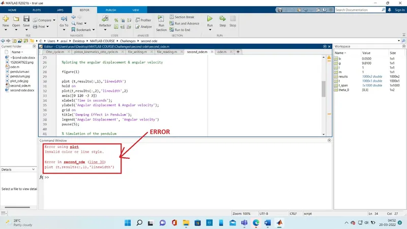
Steps were taken to correct this issue

Value of linewidth is not mentioned. Line width value=3 entered & program corrected.

Error-2

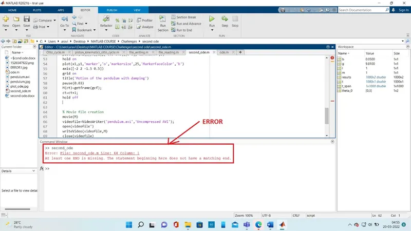
Steps were taken to correct the issue

In For loop command , end conmand is missing.

End command added in For loop & program executed.