Challenge

Project 2 - Rankine cycle Simulator

GGautham Sundararajan2 May 2022

Objective:

Create a Rankine Cycle Simulator using Matlab.
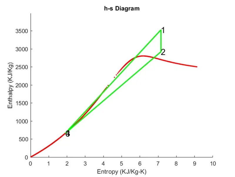
Plot the corresponding T-s & h-s diagrams.

Rankine Cycle-Explanation:

The Rankine cycle is an idealized thermodynamic cycle describing the process by which certain heat engines, such as steam turbines or reciprocating steam engines, allow mechanical work to be extracted from a fluid as it moves between a heat source and heat sink.

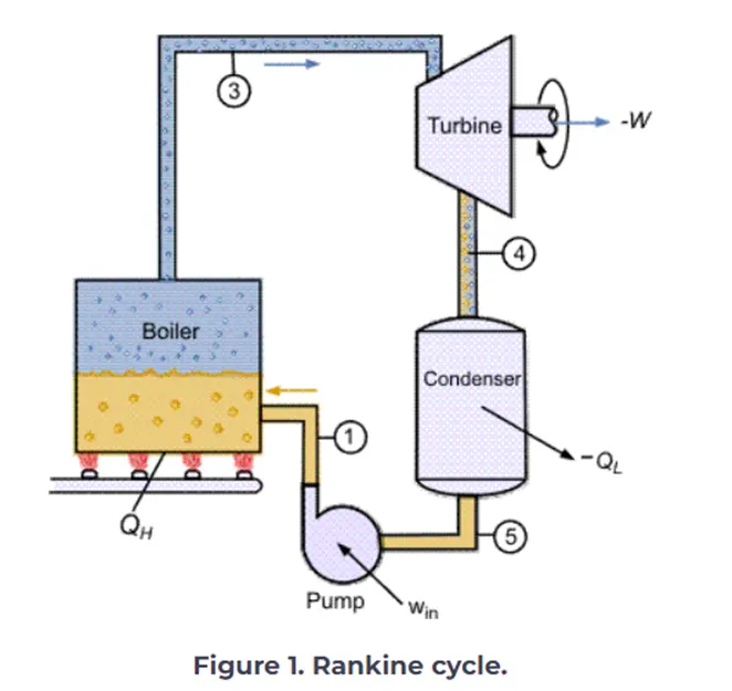
The Rankine cycle is the fundamental operating cycle of all power plants where an operating fluid is continuously evaporated and condensed. The selection of operating fluid depends mainly on the available temperature range. Figure 1 shows the idealized Rankine cycle.

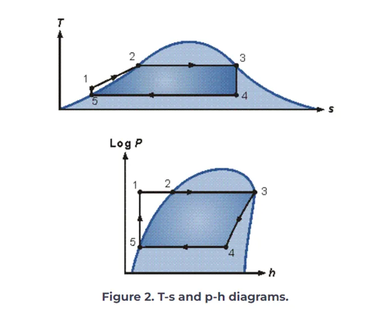
The pressure-enthalpy (p-h) and temperature-entropy (T-s) diagrams of this cycle are given in Figure 2. The Rankine cycle operates in the following steps:

1-2 Isobaric Heat Addition. High-pressure liquid enters the boiler from the feed pump (1) and is heated to the saturation temperature (2). Further addition of energy causes evaporation of the liquid until it is fully converted to saturated steam (3).
3-4 Isentropic Expansion. The vapor is expanded in the turbine, thus producing work that may be converted to electricity. In practice, the expansion is limited by the temperature of the cooling medium and by the erosion of the turbine blades by liquid entrainment in the vapor stream as the process moves further into the two-phase region. Exit vapor qualities should be greater than 90%.
4-5 Isobaric Heat Rejection. The vapor-liquid mixture leaving the turbine (4) is condensed at low pressure, usually in a surface condenser using cooling water. In well-designed and maintained condensers, the pressure of the vapor is well below atmospheric pressure, approaching the saturation pressure of the operating fluid at the cooling water temperature.
5-1 Isentropic Compression. The pressure of the condensate is raised in the feed pump. Because of the low specific volume of liquids, the pump work is relatively small and often neglected in thermodynamic calculations.

Input Values:

Turbine inlet temperature = 400 Deg C

Turbine inlet pressure = 30 bar

Turbine Outlet/ Condenser inlet pressure = 0.05 bar

Matlab code:

clear all
close all
clc

% Rankine Cycle Simulator
disp('Rankine Cyclone Simulator')
disp('1-2: Isentropic Expansion in the Turbine')
disp('2-3: Isobaric Heat Rejection by the Condenser')
disp('3-4: Isentropic Compression in the pump ')
disp('4-1: Isobaric Heat Addition by the Boiler')

t=linspace(0,400,300);

% Inputs

P1=input('Enter the pressure at the Turbine inlet (in bar)...');
T1=input('Enter the temperature at the tubine inlet (in Deg C)... ');
P2=input('Enter the pressure at the condenser (in bar)...');
disp('')

% State point-1
h1=XSteam('h_pT',P1,T1);
s1=XSteam('s_pT',P1,T1);
h_l1=XSteam('hL_p',P1);
h_g1=XSteam('hV_p',P1);
s_l1=XSteam('sL_p',P1);
s_g1=XSteam('sV_p', P1);
T_sat1=XSteam('Tsat_p',P1);


% State point -2

s2=s1;
s_l2=XSteam('sL_p',P2);
s_g2=XSteam('sV_p',P2);

% Dryness Fraction
x=(s2-s_l2)/(s_g2-s_l2);

h_l2=XSteam('hL_p',P2);
h_g2=XSteam('hV_p',P2);

% Calculating enthalpy at point 2
h2=h_l2+(x*(h_g2-h_l2));
T2=XSteam('T_ph',P2,h2);
T_sat2=XSteam('Tsat_p',P2);

% State Point-3

h3=h_l2;
s3=s_l2;
P3=P2;
T3=T2;
v3=XSteam('vL_p',P2);

% State Point-4

s4=s3;
P4=P1;
h4=XSteam('h_ps',P4,s4);
T4=XSteam('T_ps',P4,s4);
gamma=h4/T4;
r=(gamma-1)/gamma;

 % Plot

 % T-s Diagram

 figure(1)
 hold on

 % Saturation Curve
 for i=1:length(t)
     plot(XSteam('sL_T',t(i)),t(i),'r.')
     plot(XSteam('sV_T',t(i)),t(i),'r.')
 end

 % Rankine Cycle
 plot([s1 s2],[T1 T2],'lineWidth', 3, 'Color','g')
 text(s1,T1,'1','FontSize',15)

 % Beyond saturation curve

if x>1
    T3=T_sat2;
    plot ([s2 s_g2 s3 s4], [T2 T_sat2 T3 T4], 'linewidth',3,'Color','y')
    text(s2,T2,'2','FontSize',15)
    text(s_g2,T_sat2,'2s','FontSize',15)
           
% Beneath saturation curve

else
    plot ([s2 s3 s4], [T2 T3 T4], 'linewidth',2,'Color','y')
    text(s2,T2,'2','FontSize',15)
    text(s_g2,T_sat2,'2s','FontSize',15)
    
end

n=linspace(T1,T2,500);

for i=1:length(n)
    plot(XSteam('s_pT',P1,n(i)),n(i)'.','linewidth',2,'color','g')
end
text(s_g2,T_sat2,'2s','FontSize',15)
plot([s_g2 s3 ],[T_sat2 T3],'linewidth',2,'Color','b')
text(s3,T3,'3','FontSize',15,'HorizontalAlignment','Right','VerticalAlignment','top')
plot([s3 s4],[T3 T4],'linewidth',2,'Color','b')
text(s4,T4,'4','FontSize',15,'HorizontalAlignment','left','VerticalAlignment','bottom')
plot([s4 s_l1],[T4 T_sat1],'linewidth',2,'Color','b')
text(s_l1,T_sat1,'4s','FontSize',15,'HorizontalAlignment','left','VerticalAlignment','top')
plot([s_l1 s_g1],[T_sat1 T_sat1] ,'lineWidth', 2, 'Color','g')
text(s_g1,T_sat1,'1s','FontSize',15)
plot([s_g1 s1],[T_sat1 T1] ,'lineWidth', 2, 'Color','g')

xlabel('Entropy (KJ/Kg-K)')
ylabel('Temparature (K)')
title ('T-s Diagram')

% h-s Diagram
figure (2)
hold

% Saturation curve
for i=1:length(t)
    plot(XSteam('sL_T',t(i)), XSteam('hL_T',t(i)),'r.')
    plot(XSteam('sV_T',t(i)),XSteam('hV_T',t(i)),'r.')
end

% Rankine Cycle
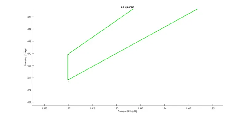
plot([s1 s2 s3 s4 s1], [h1 h2 h3 h4 h1], 'linewidth',2,'Color','g')
text(s1,h1,'1','FontSize',15)
text(s2,h2,'2','FontSize',15)
text(s3,h3,'3','FontSize',15)
text(s4,h4,'4','FontSize',15)

xlabel('Entropy (KJ/Kg-K)')
ylabel('Enthalpy (KJ/Kg)')
title('h-s Diagram')

% Calculation of desired quantities

% Work done by turbine

W_t=h1-h2;

% Work done by pump

W_p=v3*(P1-P2)*100;

% NEt work done

W_net=W_t-W_p;

% Heat Supplied

Qs=h1-h4;

% Thermal Efficiency

n_thermal=(W_net/Qs)*100;

% Back work ratio

BWR=W_p/W_t;

% Specific Steam Conductivity

SSC=3600/W_net;

% Displaying results in command window
disp('Results:-')

disp('At state point 1 :')
fprintf('P1=%.2f bar\n',P1)
fprintf('T1=%.2f Deg C \n',T1)
fprintf('h1=%.2f KJ/Kg \n',h1)
fprintf('s1=%.2f KJ/Kg-K \n',s1)
disp('')

disp('At state point 2:')
fprintf('P2=%.2f bar\n',P2)
fprintf('T2=%.2f Deg C \n',T2)
fprintf('h2=%.2f KJ/Kg\n',h2)
fprintf('s2=%.2f KJ/Kg-K \n',s2)
disp('')

disp('At state point 3:')
fprintf('P3=%.2f bar \n',P3)
fprintf('T3=%.2f Deg C \n',T3)
fprintf('h3=%.2f KJ/Kg \n',h3)
fprintf('s3=%.2f KJ/Kg-K \n',s3)
disp('')


disp('At state point 4:')
fprintf('P4=%.2f bar \n',P4)
fprintf('T4=%.2f Deg C \n',T4)
fprintf('h4=%.2f KJ/Kg\n',h4)
fprintf('s4=%.2f KJ/Kg-K \n',s4)
disp('')

fprintf('Work done by the turbine= %.2f KJ/Kg \n',W_t)
fprintf('Work done by pump=%.2f KJ/Kg\n',W_p)
fprintf('Net work done=%.2f KJ/Kg \n',W_net)
fprintf('Thermal Efficeiency=%.2fPercnet \n',n_thermal)
fprintf('Back work ratio=%f \n',BWR)
fprintf('Specific Steam Conductivity= %.2f Kg/KWh\n',SSC)

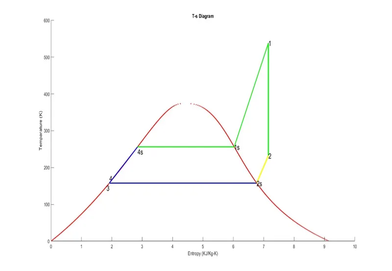
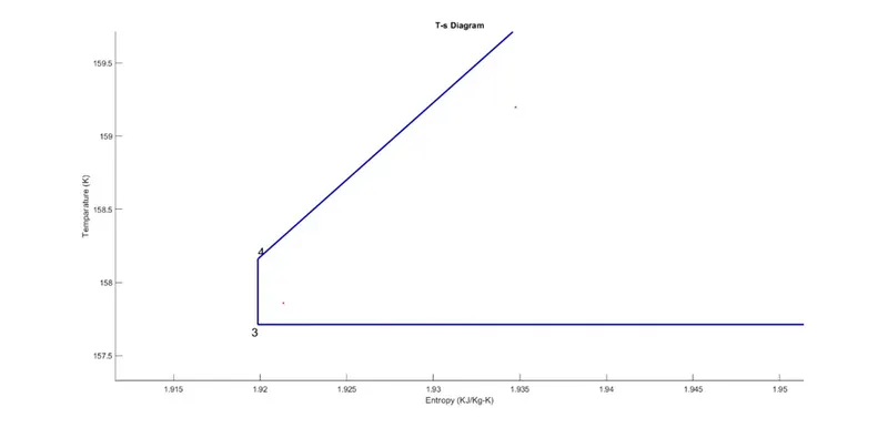
T-s Diagram:

h-s Diagram:

Stepwise procedure:

Step-1:

Click Window Start à Search ‘Matlab’ application. Once it appears on the window screen & Click the ‘Matlab’ icon.

Then Matlab application will be opened. Now first open the editor column & save the file name as ‘RankineCycle_stimulator’.

Step-2:

Enter ‘clear all, close all, ctc commands.

The usages of the commands are shown below.

‘clear all’ command is used to clear all the data stored in the workspace.

‘close all’ command is used to cleart all graphs & plots.

‘clc’ is used to clear the command window.

Step-3:

Assign the below input values.

T1=Turbine inlet temperature in Deg C

P1=Turbine inlet pressure in bar

P2=Condenser inlet pressure in bar

Step-4:

‘h_pT, s_pT, hL_p, hV_p, sL_p, sV_p, Tsat_p ‘ values are extracted from XSteam file.

Step-5:

Then, All variables from state point 1 to state point 4 extracted from XSteam file with suitable format.

Step-6:

T-s & h-s graphs are plotted from all the given values.

Step-7:

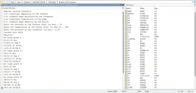
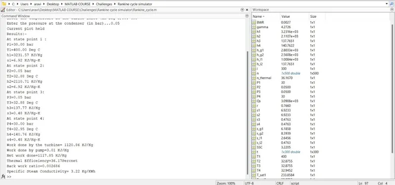
Results of the Rankine cycle simulation are displayed in a command window.

Result:

Net work done=1117.85 KJ/Kg
Back work ratio=0.002686

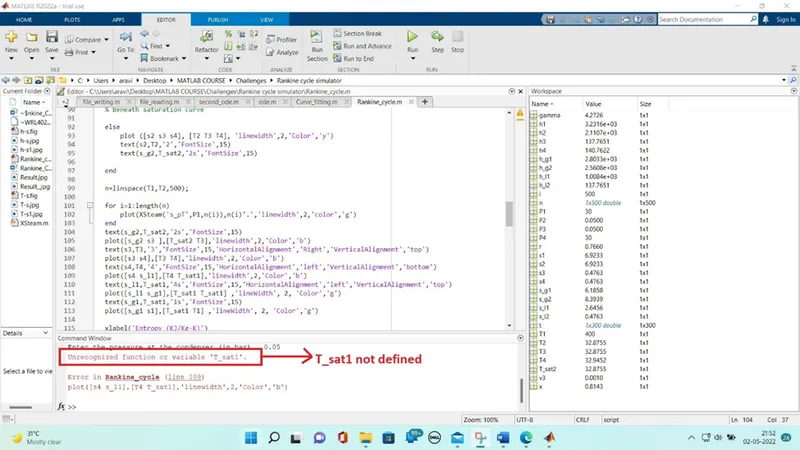
Error faced while programming:

Steps taken to correct the error:

T_sat1=XSteam('Tsat_p',P1); is assigned from XSteam file & error is corrected.

Conclusion:

The Rankine cycle plots have been generated by calculating the state points, efficiency & outputs are printed in the command window.

Reference Materials:

Project 2 - Rankine cycle Simulator

Ship work like this
in your own course.

Talk to a career counsellor

Ship work like thisin your own course.

Talk to a career counsellor

Ship work like this
in your own course.