Week 4.1 - Genetic Algorithm
AIM-
- To write a code in MATLAB to optimise the stalagmite function and find the global maxima of the function.
- To clearly explain the concept of genetic algorithm and also explain the syntax for ga in MATLAB.
- Plotting graphs for all 3 studies and for F maximum vs no. of iterations.
THEORY-
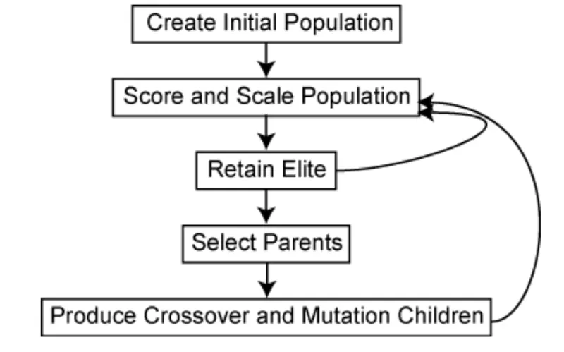
- The genetic algorithm is a method for solving both constrained and unconstrained optimization problems that is based on natural selection, the process that drives biological evolution. The genetic algorithm repeatedly modifies a population of individual solutions.
- At each step, the genetic algorithm selects individuals from the current population to be parents and uses them to produce the children for the next generation.
- Over successive generations, the population "evolves" toward an optimal solution.
- ou can apply the genetic algorithm to solve a variety of optimization problems that are not well suited for standard optimization algorithms, including problems in which the objective function is discontinuous, nondifferentiable, stochastic, or highly nonlinear.
- The genetic algorithm can address problems of mixed integer programming, where some components are restricted to be integer-valued.
- Flow chart below outlines the main algorithmic steps -
- In this study we are considering 3 cases -
- Study of GA using random sampling.
- Study of GA using lower and upper bound.
- Study of GA using lower and upper bound and increasing population size
PROGRAM/CODE-
- Below is the code to optimise the stalagmite function and find the global maxima of the function.
clear all
close all
clc

x=linspace(0,0.6,150);
y=linspace(0,0.6,150);
num_cases = 50


for i = 1:length(x)
    for j=1:length(y)
        input_vector(1) = x(i);
        input_vector(2) = y(j);
        f(i,j)=stalagmite(input_vector);
    end
end

%Study 1 -Statistical Behaviour
tic
for k = 1:num_cases
    [inputs, fopt(k)] = ga(@stalagmite,2)
    xopt(k)=inputs(1)
    yopt(k)=inputs(2)

end

study1_time = toc

figure (1)
subplot(2,1,1)
hold on
surfc(x,y,f)
shading interp
plot3(xopt,yopt,fopt,'marker','o','markersize',5,'markerfacecolor','r')
title('Unbounded Inputs')
subplot(2,1,2)
plot(-fopt)
xlabel('Iterations')
ylabel('Function Maximum ')

%Study 2 - Statistical behavior with upper and lower bounds
tic
for i = 1:num_cases;
    [inputs, fopt(i)]=ga(@stalagmite,2,[],[],[],[],[0;0],[1;1]);
    xopt(i)=inputs(1);
    yopt(i)=inputs(2);
end

study2_time = toc
figure (2)
subplot(2,1,1)
hold on
surfc(x,y,f)
shading interp
plot3(xopt,yopt,fopt,'marker','o','markersize',5,'markerfacecolor','r')
title('Bounded Inputs')
subplot(2,1,2)
plot(-fopt)
xlabel('Iterations')
ylabel('Function Maximum ')

%Study 3 - Increasing GA iterations
options = optimoptions('ga');
options = optimoptions(options,'PopulationSize',170);

tic
for i = 1:num_cases
    [inputs,fopt(i)]=ga(@stalagmite,2,[],[],[],[],[0;0],[1;1],[],[],options);
    xopt(i)=inputs(1);
    yopt(i)=inputs(2);
end

study3_time = toc
figure (3)
subplot(2,1,1)
hold on
surfc(x,y,f)
shading interp
plot3(xopt,yopt,fopt,'marker','o','markersize',5,'markerfacecolor','r')
title('Bounded Inputs with modified polulation size')
subplot(2,1,2)
plot(-fopt)
xlabel('Iterations')
ylabel('Function Maximum ')
Code 1
function [f] = stalagmite(input_vector)
f1x=(sin(5.1*pi*x+0.5))^6
f1y=(sin(5.1*pi*y+0.5))^6

f2x= exp(-4*log(2)*(x-0.667)^2)/0.64
f2y= exp(-4*log(2)*(y-0.667)^2)/0.64

f = -(f1x*f1y*f2x*f2y)

end
Code 2 - Stalagmite Function code
CODE EXPLAINATION -
- Firstly, with the help of linspace command we are defining our search space area and then finalizing the number of cases or iterations to be 50 for this study.
- Using for loop, we are creating an array of x and y values and then defining stalagmite function for plotting the stalagmite mathematical model.
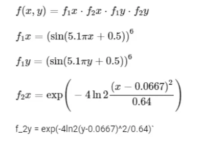
- The mathematical equation which we have used for defining our function is as below-
- In the first study which is considering random sampling, we are using GA syntax as - [x,fval] = ga(@fun,nvars)
- where x = inputs, fval = Minimum function value, fun = Function and nvars = Number of variables.
- Note - GA function always gives minimum value as the output
- By running the array of values in the for loop, we will get values of x and y where the function value is optimum.
- By plotting those values, using subplot and plot3 command we are getting our mathematical model and function values
- For results, see Figure (1)
- Since, GA gives minimum value and our aim is to find maximum function values, we just put (-ve) sign ahead of fopt and the values are plotted in reverse direction.
- In the second study which is considering the lower and upper bound sampling, we are using GA syntax as - [x,fval]=ga(@fun,nvars,A,B,Aeq,Beq,lb,ub)
- where lb = lower bound and ub = upper bound
- In this study, since we have defined our lower and upper bounds the GA will have limited interpolations to make and find the maximum function value.
- For results, see Figure (2)
- In the third study which is considering the lower and upper bound sampling with increased population size we are using GA syntax as - [x,fval]=ga(@fun,nvars,A,B,Aeq,Beq,lb,ub,nonlcon,IntCon,options)
- In this study since we have increased the population size, the GA gets more options and we get a more preciser function value.
- For results, see Figure (3)
- For all the cases we have used shading interp command so that we can get a smoother 3D curve (Stalagmite model)
- We have also used Tic and Toc command to calculate the study time. Study 3 took maximum time out of all studies.
OUTPUT RESULTS/PLOTS-
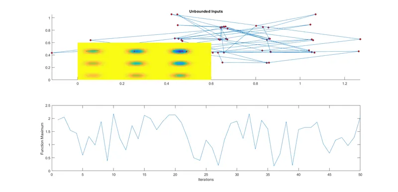
Figure 1 - Study 1 output results
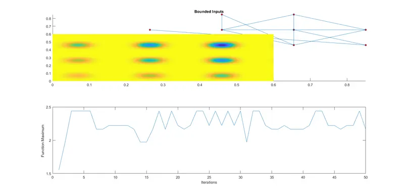
Figure 2 - Study 2 output results
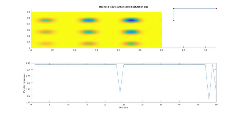
Figure 3 - Study 3 output results
ERRORS -
Error 1 - Forgot to use parantheses ().
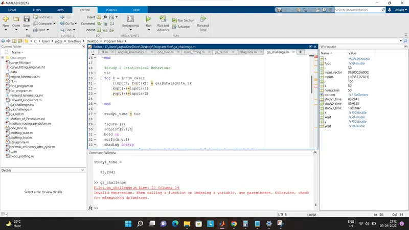
Solution - Provided parantheses at the required place.
REFERENCES -