Week 3 - Solving second order ODEs

Aim - To simulate the pendulum motion by using ode45 solver and plotting Displacement and angular velocity variation.

Solution/Code -

Below is the code for plotting Displacement and Angular velocity variation of a pendulum with respect to time -

clear all
close all
clc

%Inputs
b=0.05;
g=9.81;
l=1;
m=1;

%Initial Conditions
theta_0 = [0;3]

%Time points
t_span = linspace(0,20,500)

%Solve ODE
[t, results]= ode45(@(t,theta) ode_func(t,theta,b,g,l,m),t_span, theta_0);

%Plotting displacement and Angular velocity variation
figure(1)
plot (t,results(:,1))
hold on
plot (t, results(:,2))
xlabel('Time')
ylabel('Plot')
legend('Dispalacement','Angular Velocity')

%Using for loop for making pendulum animation
angle = results(:,1);
ct = 1;
for i = 1:length(angle)
    alpha = angle(i)
    figure (2)
    title('Motion of Pendulum')
    
    %Coordinates for the pendulum - fixed end and moving end 
    x0 = 0;
    y0= 0;
    
    x1 = l*sin(alpha);
    y1 = -(l*cos(alpha));
    
    plot([x0 x1],[y0 y1],'linewidth',3)
    hold on
    plot (x1,y1,'o','markersize',20)
    hold off
    axis([-2 2 -1.2 0])
    grid on
    pause (0.1)
    A(ct)= getframe(gcf);
    ct = ct+1;
    
end

%Making animation movie 
movie(A)
videofile = VideoWriter('Motion_of_Pendulum.avi','Uncompressed AVI');
open(videofile)
writeVideo(videofile,A)
close(videofile)

Code 1

Code 1 Explaination -

• Firstly, we have taken some input conditions for our calculations which are Damping coefficient (b) = 0.05, Gravity (g) = 9.81 m/s2, Mass (m) = 1 kg, Length (l) = 1 m, Initial displacement = 0, Angular velocity = 3 rad/s.
• We are considering the timespan of 20 seconds and dividing it in 500 divisions for visualiztion of smoother motion of pendulum.
• Now we are using ode45 solver syntax in which time (t) and theta (displacement and angular velocity) are dependent functions.
• We have also defined a function for further simplificaton of coding - ode_func(t, theta,b,g,l,m) in which the parameters mentioned in the bracket are the inputs of the functions.
• After running the code, we are getting a results matrix (500 x 2) in which the 1st column represents variation of the displacement and the 2nd column respresents variaition of the velocity.
• Now from the above result matrix, we are taking 1st column(displacement column) as our input for making the pendulum motion animation.
• Using for loop, we are running the iteration to length of the displacement column for smoother animation of the pendulum. Setting the counter initially at 1 and the running it for 500 more iterations.
• The coordinates for the pendulum are taken as x0 and y0 being fixed, and the other end of the pendulum (x1,y1) are defined using trignometry.
• Using plot command and providing the appropriate coordinates we have made the plots and then provided the axis cordinates to frame the plots properly.
• After getting all the plots and pendulum motion animation, now we are coding for making a movie of the pendulum motion. For video click here - https://drive.google.com/file/d/1zFQcjCJwxxLHQFXRsYfBuBfPtHHfKN9E/view?usp=sharing

Below is the code for the function defined for the simplification-

function [dtheta_dt] = ode_func(t,theta,b,g,l,m)
theta1= theta(1)
theta2= theta(2)
dtheta1_dt = theta2;
dtheta2_dt = -(b/m)*theta2 -(g/l)*sin(theta1);
dtheta_dt = [dtheta1_dt; dtheta2_dt];
end

Code 2 - Creating function code

Code 2 Expalaination -

• In this function we have taken t (time), theta (displacement and angular velocity),b(damping coeff), gravity, length of pendulum, mass as the input for the function.
• The second order diff equation considered is - 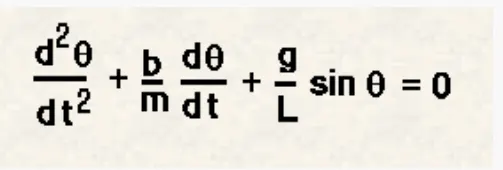----------(a)
• Now, considering Ɵ =Ɵ1

So, dƟ/dt = dƟ1/dt =Ɵ2 -----------(1)

Now,

d^2Ɵ/dt^2=d^2Ɵ1/dt^1 = d/dt(dƟ1/dt) =d/dt(Ɵ2) -----------(2)

From (a) and using (1) and (2) we have,

dƟ2/dt + b/m Ɵ2 + g/L SinƟ1 = 0

• We have created 2 ODE's which are

dƟ1/dt = Ɵ2

dƟ2/dt = -b/m Ɵ2 -g/L SinƟ1

• All the above ODE's and equations are framed in the above code.

Output Window -

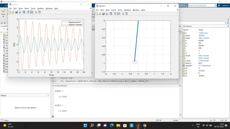
Figure 1 - Output window after running the code

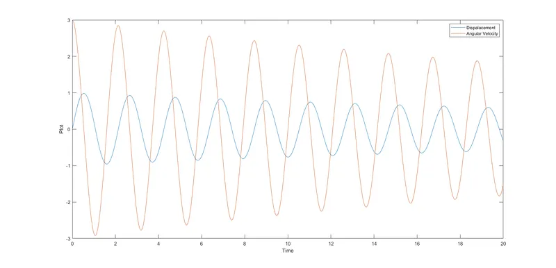
Figure 2 - Plot of Displacement and Angular velocity variation wrt time

Errors or Mistakes during coding -

• Error 1 - Considered the angle values to be in degree and therefore used Cosd and Sind, due to which the pendulum oscillation was minimal and almost not visible.

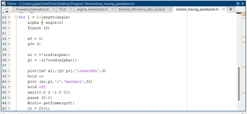
Solution - Corrected it to Cos and Sin as the angle inputs are in radians.

• Error 2 - Not using a semicolon (;) for separating the row

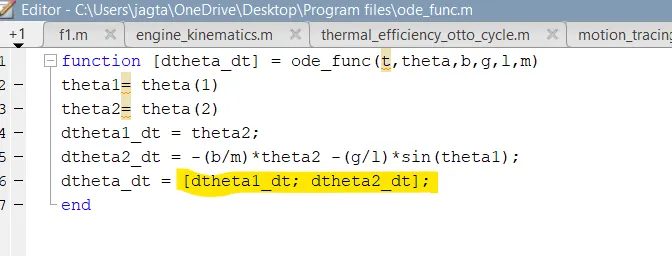
Solution - Provided the semicolon