Week 4.1 - Genetic Algorithm
GENETIC ALGORITHM

Before we move to the concept of genetic algorithm, there are some prerequisites to be understood without which Genetic Algorithm cannot be explained.
Prerequisites
1) Optimization & Optimization methods
2) Traditional optimization algorithms vs Metaheuristic algorithms
1) Optimization & Optimization methods:
Optimization:
Maximizing or minimizing some function relative to some set, often representing a range of choices available in a certain situation. The function allows comparison of the different choices for determining which might be “best.”
Common applications: Minimal cost, maximal profit, minimal error, optimal design,optimal management, variational principles
Objective function:
The objective function in a mathematical optimization problem is the real-valued function whose value is to be either minimized or maximized over the set of feasible alternatives.
Optimization methods:
Optimization methods are the methods that use a specific  algorithm to find the solution to the objective function

There are two types - Local optimization method and Global optimization method
Local optimization methods - provides result that are locally optimal, which means that it minimizes the objective function among feasible points that are near it
Examples : Nelder Mead algorithm, BFGS algorithm, Hill climbing algorithm

Global optimization methods - the algorithm searches for the global optimum by employing mechanisms to search larger parts of the search space.
Examples : Genetic algorithm, Simulated Annealing, Particle Swarm Optimization.
2) Traditional optimization algorithms vs Metaheuristic algorithms
Metaheuristic algorithms are not problem dependent, this means that they can be used for any optimization problem unlike traditional optimization algorithms.
Advantages of Metaheuristic algorithms over traditional optimization algorithms
i) Speed and problem size:
Metaheuristic algortithms is faster than traditional algorithms and can handle larger problems.
ii) Local minima and global minima:

From the above plot, f(x) is the objective function that has to be minimised for the best value. x1 is the local minima and x2 is the global minima.0

Traditional algorithms terminate at local minima.
As the algorithm search starts , it looks for the best answer i.e, to minimise f(x). It reaches x1 (let us say x1 = 4) and f(x1) will be the minimum, the search moves to next value where f(x=4.1) and this gives an f(x) less than f(x1). Now, the search algorithm stops or terminates  here and would return x1 = 4  as the best value. This is because the traditional algorithm would update only best values would not consider worst values. As it moves ahead, i.e., > x1, the f(x) obtained is > f(x1) and the search terminates as it considers x1 as the best one and doesn't accept any value greater than x1. Therefore, there is a high probability of returning local minima as the best values.
Metaheuristic algorithms won't terminate at local values.
Metaheuristic algorithms avoid getting stuck in a local minima and escape it because it uses randomness (or random numbers) to accept worse moves (larger f(x) for minimization problems) because they may lead to better answers (i.e. a better local minima or a global minima). The search algorithm accepts worse values than x1=4 and moves on with the search, finds the global minima i.e, x2=7(say) and returns it as a best value.
iii) Neighbourhood search vs Population based search.
Neighbourhood search: In neighborhood search,  there is only one point or solution throughout the search space and it updates that solution as the algorithm  moves ahead.
Examples: Simulated annealing and tabu search.

Population based search: The algorithm evaluates all points in the population at once and generates all the solutions at once.
when the algorithm terminates, the best solution is selected from the last update in which it converged to, or, keep track of all updates and select the best out of all.

Population-based search algorithms tend to be very powerful as it explores various points in the search space rather than one.
Examples : Genetic algorithm.
GENETIC ALGORITHM
GA is a population-based metaheuristic developed by John Holland in the 1970s. GA uses techniques inspired from nature, more specifically evolution, to find an optimal or near-optimal solution towards a problem. It applies evolution concepts such as reproduction and survival of the fittest to solve a problem. GA belongs to the larger class of evolutionary algorithms.
Genetic Algorithm Flow Chart

Step 1:
Population is initialised – A population of sample data points for a variable is initialised. Let us say an objective function is a function of single variable and has a population size of 20. A number of 20 sample data points of that variable will be available in the search space. In Matlab, default of population size is 50. Random number generator is used to generate population which is in the range of 0 to 1.
for eg: population size: 3, variables : 2
population = rand(3,2)
Population = 0.0149  0.0858
          0.3852  0.9966
          0.3954  0.4020
Step 2:
Evaluation of fitness:
The GA algorithm evaluates the objective function using all the data points in the search space and a solution space is generated. For every data point, there is one solution. For a population size of 50, there will be 50 solutions.
Step 3:
Selection:
There are two ways of selecting the solutions, Tournament selection and Roulette wheel selection
Tournament selection:
Select k solutions at random from the solution space.
Pick the variable that gives the best f(x), if more than one solution tied for best, pick any and set as parent 1.
Repeat to find parent 2.

Roulette wheel selection:
Sum up all the solutions
Divide each solution by the sum to obtain probability set.
Take cumulative probability to obtain a set with range of 0 to 1.
For eg:

Variable x	f(x)	Probability	Cumulative probability	Range
2	4	0.1379	0.1379	0 ≤rand ≤0.1379
3	9	0.3013	0.4392	0.1379 ≤rand ≤0.4392
4	16	0.5517	1	0.4392 ≤rand ≤1
sum	29

To get the probabilities for each solution, we add all the fitness values (f(x)) together to get the total and divide each f(x) by the total to get a percentage of how much it occupies from the total. Then, we select a random number, which is between 0 and 1, and select the solution to be parent 1 from the probabilities set. If the 3 solutions get probabilities 13.79%, 30% and 55%, based on their fitness, and if random number comes out to be 0.65, then it will be in the range of 0.4392 and 1.00 which would make us choose the variable x =4, which had a probability of 55% of being selected. Two parents are selected for the next operation.
Step 4: Crossover
Crossover operator is used create offspring or children. There are many ways to do crossover, the most common methods are
i)	Single point cross over
  Parent 1
E 	R	T	Y	U	O

  Parent 2
S	D	F	G	H	K

  Child 1
E 	R	T	G 	H	K

  Child 2
S	D	F	Y	U	O

Here, the cut off point is at integer 3 i.e, the exchange happens after cell 3 of the parents 1 and 2. The integer is selected randomly and is considered as cutoff point
Two point crossover
  Parent 1
E 	R	T	Y	U	O

  Parent 2
S	D	F	G	H	K

  Child 1
E 	R	F	G 	H	K

  Child 2
S	D	T	Y	U	O
Here, instead of single cutoff point, two cutoff points are created by random selection of two integers and exchange happens what is in between the cutoff points. The cutoff points are at integers 2 and 4.
Step 5: Mutation
Mutation operator is used to create diversity in search space. Mutation is applied on the children after crossover. Let us consider binary numbers for example
Child 1
1	1	0	1	0	1	0	0
Child 2
1	1	0	1	0	1	0	0
Mutated Child 1
1	1	1	1	0	1	1	0
Mutated Child 2
1	0	0	1	1	1	0	0

In mutation process, if the value 0 is to be mutated, it would become 1, and if the value 1 is to be mutated, it would become a 0. In this way, the mutation children will be generated.
Now, The two individuals or sample data points of variable in the old generation population is replaced with this new population to form a new generation. To completely replace the old population with new population, the process should be repeated n/2 times from step 3 to step 5 where n is the population size.
For eg. If population size is 20, two parents are selected and undergo crossover and mutation and two mutation children or new population is generated. These two replace the old ones in the population. For each process i.e., from step 3 to step 5, two children are generated. Therefore, the process from step 3 to step5 is repeated for 20/2 = 10 times to completely create a new population.
Once the new population is created, it checks for optimal solution, if found , the algorithm terminates. If not found, the cycle repeats.
Elitism approach in GA
The other approach employed in working of GA is elitist approach. Here, the fittest individuals are selected from the solution space and are moved to next generation without any crossover or mutation. The remaining individuals in the population are subjected to crossover and mutation and subsequently new generation is created. Matlab employs elitist approach in GA.
PROGRAM TO OPTIMIZE STALAGMITE FUNCTION USING GA
Stalagmite function code

% stalagmite function =
% (sin((5.1*pi)*x(1)+0.5))^6*(sin((5.1*pi)*x(2)+0.5))^6*exp((-4*log(2))*(x(1)-0.0667)^2/(0.64))*exp((-4*log(2))*(x(2)-0.0667)^2/(0.64))

% code to generate stalagmite function, x is an input vector with elements
% x1 and x2

function f = stalagmite(x)
f1 = (sin((5.1*pi)*x(1)+0.5))^6;

f3 = exp((-4*log(2))*(x(1)-0.0667)^2/(0.64));

f2 = (sin((5.1*pi)*x(2)+0.5))^6;

f4 = exp((-4*log(2))*(x(2)-0.0667)^2/(0.64));


f = -(f1*f2*f3*f4);
end


Optimization Program Code
clear all
close all
clc
 x = linspace(0,0.6,150);
 y = linspace(0,0.6,150);
 % x and y vectors are created using linspace command with ranging from 0
 % to 0.6 with 150 equal intervals. size of each vector

 [xx yy] = meshgrid(x,y);
 % x and y vectors are converted to matrices xx and yy(using meshgrid command) of size 150x150 each
 % to form a mesh grid

 for i = 1:length(xx)
     for j = 1:length(yy)
     input_vector(1) = xx(i,j);
     input_vector(2) = yy(i,j);
     zz(i,j) = stalagmite(input_vector);

     end
 end


% for loop of i takes on values from 1 to 150 along the length of xx matrix.
% for loop of j takes on values from 1 to 150 along the length of yy matrix.
% xx(i,j) is the index of xx matrix and is assigned a variableinput_vector(1).
% yy(i,j) is the index of yy matrix and is assigned a variable input_vector(2).
% z(i,j) is the index of z matrix, each element of the matrix is returned by stalagmite
% function and the input vector(1) and input_vector(2) are the input arguments to that function.
% for each value of i, j value moves from 1 to 150 and therefore z matrix of size 150x150 is generated

% Using genetic algorithm to find the minimum of the objective function.
% Our aim here is to find the maximum of the function the objective function. Therfore, we multiply our objective function with a negative sign.
% Objective function here is stalagmite function.(is multiplied with a negative sign to find the maximum of the function)
% Our objective function here has no contraints.

num_cases=50;
% let us consider the no of iteration for genetic algorithm to run be 50
% and is assigned a variable num_cases

% Case 1 - Unbounded inputs
% let us consider no bounds for input variables and perfrom ga on the
% objective function
 tic
 % tic - starts the stopwatch timer
 for i=1:num_cases
     [u,F(i)]=ga(@stalagmite,2);
     h(i)=u(1);
     g(i)=u(2);

 end
 studytime1=toc
% toc calculates the elapsed time - taken for the program to run

% GA SYNTAX for case 1
% [x,fval]=ga(fun,nvars) -
% u=x,F(i)=fval,@stalagmite=fun,nvars=2.
% ga returns the best values of input variables for which the objective function is minimum/maximum (maximum in our program)
% fun - objective function (stalagmite function in our program)
% nvars - no of input variables with no bounds
% x - returns input variables or the best values for which the objective
% function is maximum
% fval - returns maximum function value

% for loop
% for loop of i, it takes values from 1 to 50. u is an input vector of which u(1) returns input variable 1 and u(2) returns input variable 2.
% u(1) is assigned a variable h(i), an index of an element from vector h,
% for 50 iterations of ga, 50 entries of input variable 1 will be generated in 'h' vector forming a vector of size 1x50
% similarly procedure for generation of vector 'g'
% for 50 iterations of ga, 50 entries of function value 1 will be generated in 'F' vector forming a vector of size 1x50

figure(1)
 subplot(2,1,1)
 % generates plot in a 2x1 vector that is positioned at first row and first column
 hold on;
 % holds on the plot
 surfc(xx,yy,-zz);
 % generates a 3D plot or surface plot of z over xx and yy meshgrid. -zz is
 % generates a surface plot of peaks to find the maximum using ga.
 shading interp;
 %sahding interp varies the color in each line segment and face by interpolating the colormap index or true color value across the line or face.
 plot3(h,g,-F,'Marker','o','MarkerSize',5,'MarkerFaceColor','r')
 % generates a 3D plot line with h and g as x and y axes and F as z axis.
 % -F is to search for the maximum of the function. If we use +F, it will
 % search for the minimum.
 title('Unbounded inputs')
 % creates a title for the subplot

 subplot(2,1,2)
 % generates plot in a 2x1 vector that is positioned at second row and first column
 plot(-F)
 % generates a 2D plot with -F on y axis and no of values of -F or iterations on x axis
 xlabel('Iterations')
 % generates xlabel for the subplot
 ylabel('F maximum')
 % generates ylabel for the subplot
 title('F max vs Iterations')
 % creates a title for the subplot


% Repeating the same procedure as Case 1 but with bounds for inputs
% Case 2 - Bounded inputs

 tic
 for i=1:num_cases
     [u,F(i)]=ga(@stalagmite,2,[],[],[],[],[0;0],[1;1]);
     h(i)=u(1);
     g(i)=u(2);

 end
 studytime2=toc


% GA SYNTAX for Case 2
% [x,fval]=ga(fun,nvars,A,b,Aeq,beq,lb,ub)
% A*x<=b - linear inequality constraints = nil for our objective function
% Therefore, A = [], b = []
% Aeq*x=beq - linear inequality constraints = nil for our objective function
% Therefore, Aeq = [], beq = []
% lb = lower bounds for the input variables - [0;0] for both input variables
% up = upper bounds for the input variables - [1;1] for both input variables

 figure(2)
 subplot(2,1,1)
 hold on;
 surfc(xx,yy,-zz);
 shading interp;
 plot3(h,g,-F,'Marker','o','MarkerSize',5,'MarkerFaceColor','r')
 title('Bounded inputs')

 subplot(2,1,2)
 plot(-F)
 xlabel('Iterations')
 ylabel('F maximum')
 title('F max vs Iterations')


% Repeating the same procedure as Case 2 but with bounds for inputs and increased population size
% Case 3 - Bounded inputs with increased population size


 options=optimoptions('ga','PopulationSize',300)
 % sets the initial population size to 300 for the ga. The default initial population size considered by ga is 50.
 tic
 for i=1:num_cases
     [u,F(i)]=ga(@stalagmite,2,[],[],[],[],[0;0],[1;1],[],[],options);
     h(i)=u(1);
     g(i)=u(2);

 end
 studytime3=toc

% GA SYNTAX for Case 3
% [x,fval]=ga(fun,nvars,A,b,Aeq,beq,lb,ub,nonlcon,intcon,options)
% A*x<=b - linear inequality constraints = nil for our objective function
% Therefore, A = [], b = []
% Aeq*x=beq - linear inequality constraints = nil for our objective function
% Therefore, Aeq = [], beq = []
% lb = lower bounds for the input variables - [0;0] for both input variables
% up = upper bounds for the input variables - [1;1] for both input variables
% nonlcon - nonlinear contraints = nil for our objective function = []
% intcon - integer constraints = nil for our objective function = []
% options - defined for a poplualtion size of 300

 figure(3)
 subplot(2,1,1)
 hold on;
 surfc(xx,yy,-zz);
 shading interp;
 plot3(h,g,-F,'Marker','o','MarkerSize',5,'MarkerFaceColor','r')
 title('Bounded inputs - Population size 300')


subplot(2,1,2)
 plot(-F)
 xlabel('Iterations')
 ylabel('F maximum')
 title('F max vs Iterations')


Stopping Criteria for Genetic Algorithm
•	When there has been no improvement in the population for X iterations.
•	When we reach an absolute number of generations.
•	When the objective function value has reached a certain pre-defined value.
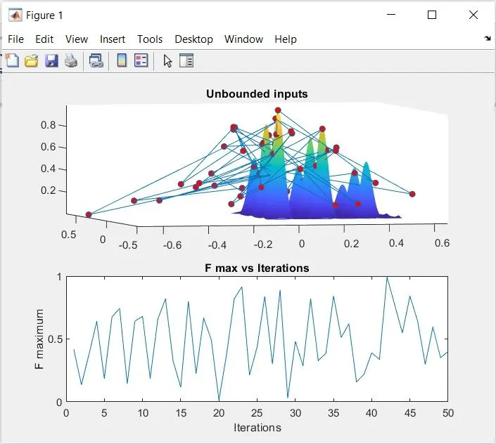
Output plot for Case 1 - Unbounded inputs
Observations
From the plot, it is evident that the ga is considering all types of inputs i.e., the sample data points from the search space and is not going in the proper direction to find the maximum of the objective function.
Reason:
1) The inputs are not bounded (since the inputs are not bounded, ga considers all kinds of random inputs and may not move in the right direction to find the maxima)
2) The default population size considered by ga is 50 ( less size to find the accurate solution)
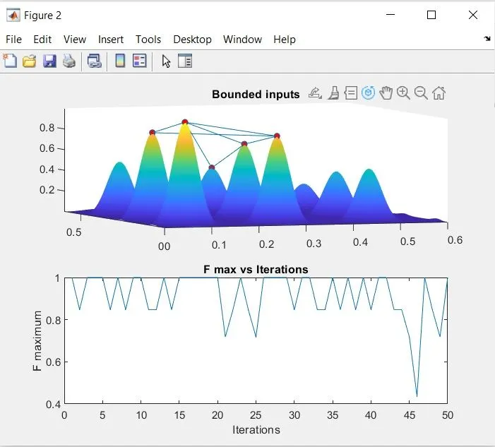
Outplot for Case 2 - Bounded Inputs
Observations
From the plot, it is evident that the ga is searching and moving from one maxima to another. This shows that ga is moving in proper direction to find the maxima compared to case 1.
Reason:
1) The inputs are bounded (since the inputs are bounded, ga searches the inputs in a limited space may move in the right direction to find the maxima)
2) The default population size considered by ga is 50 ( less size to find the accurate solution)
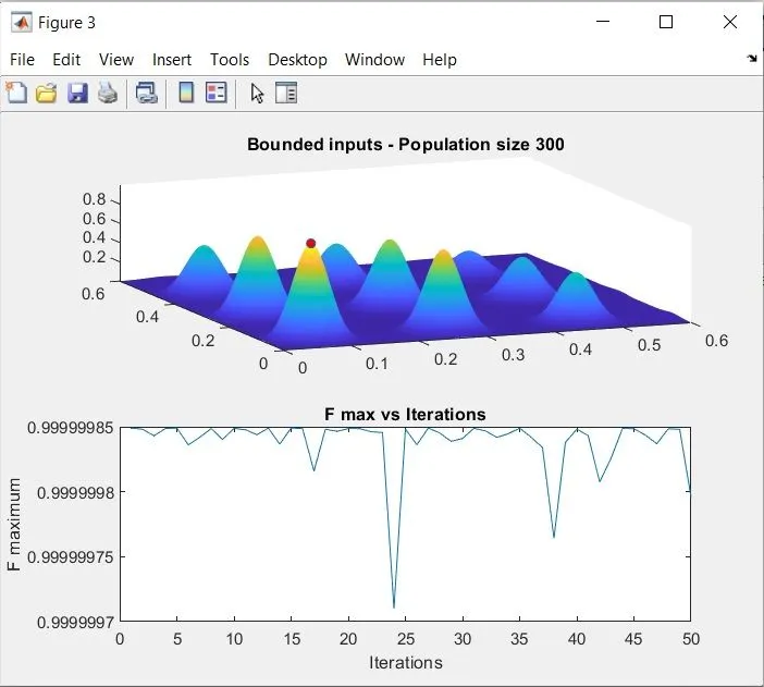
Outplot for Case 3 - Bounded Inputs & Increased population
Observations
From the plot, it is evident that the ga has converged to an optimal solution that leads to the global optima of the function. This shows that ga has searched and moved in proper direction to find the maxima compared to case 1 & case 2.
Reason:
1) The inputs are bounded (since the inputs are bounded, ga searches the inputs in a limited space may move in the right direction to find the maxima)
2) The population size has been increased to 300 ( much greater than the default size of 50, as the population is increased,diversity increases, the probability to find the accurate solution is high)
The program has been executed many times and solution obtained for the case 3 remained same.
Study times
Case1 = 4.1368, Case2 = 3.9387, Case3 = 13.0492
The study times for case 1 and case 2 are almost close and the slight variation could be due to the unbounded nature of case1 compared to case2. The study time for case3 is high due to the high population size compared to case1 and case2.
More the population, more the function evaluations and therefore more the time.
'Stalagmite program and function files are attached'
References
1) Genetic Algorithm (GA): A Simple and Intuitive Guide | by Dana Bani-Hani | Towards Data Science.
2) Local Optimization Versus Global Optimization by Jason Brownlee.
3) Genetic algorithm options, terminology and working - matlab help
4) Variations of Genetic Algorithm by Alison Jenkins, Vinika Gupta, Alexis Myrick, and Mary Lenoir