Week 3 - Solving second order ODEs
clear all
close all
clc


% Assigning input variables
% lenght of pendulum = l(m)
l = 1;
% damping coefficient = b
b = 0.05;
% mass of ball= m(kg)
m = 1;
% acceleration due to gravity = g(m/s2)
g = 9.81;

% initial conditions for angular displacement and angular velocity
theta_0 = [0 3];
% theta_0 is a column vector as the differential equations to solved is
% also a column vector

% Time given to simulate the motion is o to 20 seconds
t_span = linspace(0,20,200);
% Use of linspace command to to divide 0 to 20 into 200 equal intervals for
% smooth transitions from one frame to the other

% Using ode45(built in solver) to solve the differential equations
[t,results] = ode45(@(t,theta)ode_func(t,theta,b,g,l,m),t_span,theta_0)

% Syntax explanation
% [t, results] - Output variables returned by the solver ode45, results is
% the solution matrix that consists of two arrays(column vectors) - one is
% angular displacement and the other is angular velocity.
% the solution matrix returns a value for each value of t in the column
% vector of t (i.e., for each value of t, an output will be returned for
% angular displacement and angular velocity)


% ode45(@(t,theta) ode_func(t,theta,b,g,l,m),t_span,theta_0)
% ode45 is a solver that integrates a system of differential equations
% The differential equations to be solved in this problem are
% 1) dtheta1_dt = theta2
% 2) dtheta2_dt = -(b/m)*theta2-(g/l)*sin(theta1) (refer ode_func file for ref.)

% @(t,theta)
% an anonymous function call that defines and tells the solver that
% differential equation has two inputs i.e., t and theta. t - independent
% variable and theta - dependent variable. theta is a function of t.

% ode_func(t,theta,b,g,l,m)
% ode_func is a function that defines the functions or system of differential equations to be integrated or to be solved by ode45
% It has input arguments other than t and theta i.e., b,g,l and m. These inputs have predefined values. While
% solving, the predefined values will be passed on to b,g,l and m that are defined in ode_func.

% (theta_0,t_span)
% theta_0 represents initial conditions for angular displacement and
% angular velocity so that the solver computes the constant value and
% genetrates  solution equations.
% t_span represents time points ranging from 1 to 20 and the solver computes and outputs
% the angular displacement and angular velocity for each time point in t
% array


figure(1)
plot(t,results(:,1),t,results(:,2))
% creates a plot for results of angular displacement(1st column of results matrix) & angular velocity(second column of results matrix) of pendulum vs time
% ranging from 0 to 20 seconds
xlabel('time')
% labels x axis
ylabel('plot')
% labels y axis
title("Variation of Ang disp and Ang vel w.r.t Time")
% diplays title on top of the plot
legend('ang disp','ang vel')
grid on

% Animation of simple pendulum motion
%assigning variable to angular diplacement solution array
ang_disp = results(:,1);
ct=1;
% ct represents counter for each plot or frame
for i=1:length(ang_disp)
    % for loop is initiated, condition - variable 'i' goes through the no of values
    % assigned ang_disp i.e., a total of 200 values. Therefore, the
    % instructions or commands in the for loop are repeated 200 times, A
    % total of 200 plots/frames are generates showing different positions of
    % pendulum at different times

    K=ang_disp(i);
    % K takes values assigned to ang_disp array i.e.,
    % ang_disp(1),ang_disp(2)....ang_disp(200)

    l = 1;
    % length of pendulum(m)
    x0 = 0;
    y0 = 0;
    % (x0,y0) respresents fixed point of pendulum from which it hangs
    x1 = l*sin(K);
    y1 = -l*cos(K);
    % (x1,y1) represents the end point of pendulum length that is free to
    % move and on which the ball is fixed.
    % From trigimoetric approach, x1=lsink - projection of l on x axis in positive x direction
    % From trigonometric approach, y1=-lcosk - projection of l on y axis in negative y direction

    figure(2)

    % holds the plot
    plot(x1,y1,'o','markersize',20,'markerfacecolor','g')
    hold on;
    % plots the marker that is made to appear as a ball of the pendulum at
    % the free end, marker size is 20 and its face color is green.
    plot([x0 x1],[y0 y1],'color','b','linewidth',3)
    % creates a plot of the length of string of pendulum that varies its
    % position w.r.t time., color of plot is blue and width is 3.
    hold off;
    % holds off the plot
    xlabel('x axis')
    ylabel('y axis')
    grid on
    title('Motion of Simple Pendulum - MATLAB')
    legend('ball','length of string')

    axis ([-2.5 2.5 -2.5 2.5])
    % limits the x axis (-3 3) and y axis (-3 3)
    pause(0.1)
    % pauses the program execution for 0.1 seconds after each run
    M(ct)=getframe(gcf);
    % M - array of frames
    % getframe - records or captures plot, each plot is one frame
    % gcf - gets  the current figure or plot that is being executed
    ct = ct+1;
    % after counter 1, it increments by one to execute the program for next plot
    % and so on till the for loop terminates
end
% end of for loop
movie(M)
% movie - to play movie file with M array of frames
Videofile=VideoWriter('Test_shm.avi','Uncompressed AVI')
% Videowriter creates a videofile and file format on which video data can be written
% videofile is the name or variable assigned to videowriter
open(Videofile)
% opens the videofile for writing video data
writeVideo(Videofile,M)
% writevideo - writes the video data of M i.e., the frames captured by M onto the videofile
close(Videofile)
% closes the videofile after writing video data
FUNCTION FILE - ode_func
The function file(ode_func) is attached in the attachments
Errors faced while programming
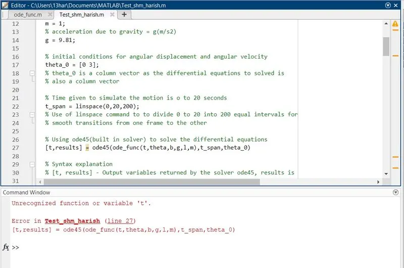
syntax error - did not mention inputs of the function i.e., t,theta
t and theta should be mentioned as inputs and specified as an anonymous function in the ode45 function call
corrected syntax [t, results] = ode45(@(t,theta)ode_func(t,theta,b,g,l,m),t_span,theta_0)
OUTPUT 1 - PLOT
Explanation
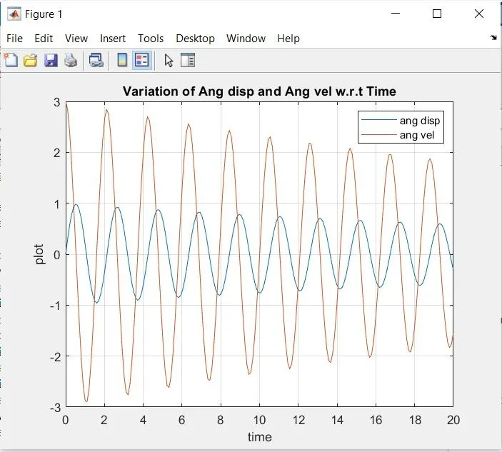
As observed from the plot, the blue curve represents angular displacement , red curve represents angular velocity and both are varying w.r.t time.
The angular velocity of the pendulum is reducing as time marches forward. This is due to presence of damping. The damping coefficient provide is 0.05. The damping can be due to air resistance that decreases the velocity of pendulum. As the velocity of the pendulum decreases, the displacement of the pendulum also decreases (also seen from the plot) and therefore, the oscillations die out or the pendulum complelely comes to rest.
Since, we have considered to observe the oscillations for a time range of 0 to 20 seconds, as can be seen from the plot, the oscillations did not dampen completely or came to a complele zero or no oscillations. If we increase the time range, we can observe at what time oscillations are completely dying out.
The other way is to increase the damping coefficient keeping the time range constant observe the time at which oscillations are dying out completely with in 20 seconds range.
OUTPUT 2 - MOTION PLOT
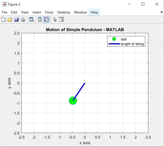
The above figure generates a motion plot (a total of 200 plots) with a pause of 0.1 seconds for each plot generation.
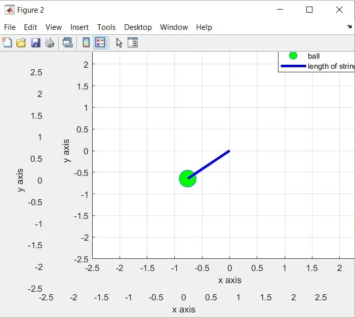
The above figure shows the movie animation with M - an array of frames or plots(200) with default fps of 12
OUTPUT 3 - ANIMATION VIDEO FILE
The youtube link to the animation video file (30fps) is attached below