Project 2 - Rankine cycle Simulator
Project 2 - RANKINE CYCLE SIMULATOR
Vapour Power Cycle
Vapour power cycles are power cycles used in steam power plants. In a power cycle, heat energy (released by the burning of fuel) is converted into work (shaft work), in which a working fluid repeatedly performs a succession of processes. In a vapour power cycle, the working fluid is water, which undergoes a change of phase.
In a vapour power cycle, the working fluid is subjected to change in its properties in different stages of the cycle. Heat is transferred to water in the boiler from an external source(furnace where fuel is continuously burnt) to raise steam (mass of water = 1kg). The high pressure, high temperature steam leaving the boiler expands in the turbine to produce shaft work, the steam leaving the turbine condenses into water in the condenser( where cooling water circulates) rejecting heat, and then the water is pumped back to the boiler.
Since the fluid is undergoing a cyclic process, there will be no net change in its internal energy over the cycle, and consequently the net energy transferred to the unit mass of fluid as heat during the cycle must equal the net energy transfer as work from the fluid (from First Law of Thermodynamics)
∑Qnet cycle =∑Wnet cycle
Q1-Q2 = WT - WP
Q1 = heat transferred to the working fluid (kJ/kg)
Q2 = heat rejected from the working fluid (kJ/kg)
WT = work transferred from the working fluid (kJ/kg)
WP = work transferred into the working fluid (kJ/kg)
The efficiency of vapour cycle is
Ղ = Wnet/Q1 = WT – WP/Q1
Rankine Cycle
For each process in vapour power cycle, an ideal process is assumed to get an estimate of the ideal or maximum efficiency of the cycle. Since all processes are ideal, the cycle becomes an ideal cycle called as Rankine cycle. The T-S diagram for ideal rankine cycle is as follows.
In the ideal cycle, working fluid at outlet of boiler can be in mixed phase (liquid and vapour), dry saturated vapour or super heated steam.
The working fluid passes through four engineering systems or devices in the cyclic process. They are boiler, turbine, condenser and pump. Each system or device is a considered as an open system i.e., assumed as a control volume through which working fluid undergoes mass and energy interactions across the system boundary or control surface.
Work done calculations
Work done in open system is Flow work = ʃ Vdp
Heat and Work indications
Work done on the system – negative sign (-W)
Work done by the system – positive sign (W)
Heat supplied to system – positive sign (Q)
Heat rejected by system – negative sign (-Q)
For analysis of Rankine cycle, considering the flow of working fluid to be steady along all the engineering devices. The steady flow energy equation (S.F.E.E.) for a fluid passing through or entering and leaving a control volume is given by
h1+V12/2+Z1g+dQ/dm = h2+V22/2+Z2g+dWx/dm
(properties of working fluid at entrance) = (properties of working fluid at exit)
h – enthalpy/unitmass kJ/kg
V2/2 – Kinetic energy/unitmass kJ/kg
Zg – Potential energy/unitmass kJ/kg
dQ/dm – net heat transfer per unit mass through the control surface kJ/kg
dWx/dm – net work transfer per unit mass through the control surface kJ/kg
Applying S.F.E.E. to all processes in Rankine cycle
Mass of fluid = 1kg
Neglecting change in KE and PE for all the processes i.e.,
V22/2- V12/2 = 0 and Z2g- Z1g = 0 and evaluating the heat and work interactions.
Process 1-2: Isentropic Expansion Process
Work done on turbine by the working fluid
h1=Wt+h2
Wt=h1-h2
Wt – work done on turbine
Process 2-3: Constant Pressure heat rejection process
Heat rejection from working fluid in condenser
h2-Qr=h3 (heat rejected from the system ,therefore, Q is –ve)
Qr=h2-h3
Qr – heat rejected from condenser
Process 3-4: Isentropic Compression Process
Work done by pump on the working fluid
h3=-Wp+h4 (work done on the system, therefore, W is –ve)
Wp=h4-h3
Wp – work done by pump
Process 4-1: Constant Pressure heat addition process
Heat supplied to working fluid by boiler
h4+Qs=h1
Qs=h1-h4
Qs – heat supplied by boiler
clear all
close all
clc

fprintf('                   RANKINE CYCLE SIMULATOR                             \n')
fprintf('1-2 is Isentropic Expansion of working fluid Turbine\n')
fprintf('2-3 is Constant pressure heat rejection from working fluid in condenser\n')
fprintf('3-4 is Isentropic compression of working fluid in pump\n')
fprintf('4-1 is Constant pressure heat addition to working fluid in boiler\n\n')

p1=30;
p2=0.05;
T1=400;

fprintf('Pressure of working fluid at the inlet of turbine (bar) : %f \n',p1)
fprintf('Pressure of working fluid at the outlet of turbine (bar) : %f\n',p2)
fprintf('Temperature of working fluid at the inlet of turbine (deg C) : %f\n\n',T1)

h1=XSteam('h_pT',p1,T1);
s1=XSteam('s_pT',p1,T1);

s2=s1;

sl2=XSteam('sL_p',p2);
sg2=XSteam('sV_p',p2);
hl2=XSteam('hL_p',p2);
hg2=XSteam('hV_p',p2);

X2=(s2-sl2)/(sg2-sl2);

h2=(hg2-hl2)*X2+hl2;

T2=XSteam('T_hs',h2,s2);

p3=p2;
p4=p1;
T3=T2;

h3=XSteam('hL_p',p3);
s3=XSteam('sL_p',p3);
v3=XSteam('vL_p',p3);

s4=s3;

Cp4=XSteam('Cp_ps',p4,s4);
Cv4=XSteam('Cv_ps',p4,s4);
gamma = Cp4/Cv4;
r = (gamma-1)/gamma;
T4=T3*(p4/p3)^r;

W_P=v3*(p4-p3)*100;
h4=h3+W_P;

W_T=h1-h2;
W_net=W_T-W_P;
Q_boiler=h1-h4;

ntherm=W_net/Q_boiler*100;
Backworkratio=W_P/W_T;
Steamrate=3600/W_net;


T5=XSteam('Tsat_p',p1);
T6=T5;
s5=XSteam('sL_p',p1);
s6=XSteam('sV_p',p1);

T_satcurve=linspace(1,500,500);
for i=1:length(T_satcurve)
    sL(i)=XSteam('sL_T',T_satcurve(i));
    sV(i)=XSteam('sV_T',T_satcurve(i));
end
subplot(1,2,1)
hold on;
plot([s1 s2 s3 s4 s5 s6 s1],[T1 T2 T3 T4 T5 T6 T1],'lineWidth',1.5,'color','b')
plot(sL,T_satcurve,'lineWidth',1.5,'color','r')
plot(sV,T_satcurve,'lineWidth',1.5,'color','r')
axis([0 10 0 500])
xlabel('Entropy [kJ/kgK]')
ylabel('Temperature [K]')
title('T-S plot for Rankine cycle')
legend('TS rankine','Satcurve')


text(s1,T1,'1','FontSize',10)
text(s2,T2,'2','FontSize',10)
text(s3,T3,'3','FontSize',10,HorizontalAlignment='left',VerticalAlignment='top')
text(s4,T4,'4','FontSize',10,HorizontalAlignment='right',VerticalAlignment='top')

h5=XSteam('sL_p',p1);
h6=XSteam('sV_p',p1);
for i=1:length(T_satcurve)
    hL(i)=XSteam('hL_T',T_satcurve(i));
    hV(i)=XSteam('hV_T',T_satcurve(i));
end

subplot(1,2,2)
hold on;
plot([s1 s2 s3 s4 s1],[h1 h2 h3 h4 h1],'lineWidth',1.5,'color','g')
plot(sL,hL,'lineWidth',1.5,'color','r')
plot(sV,hV,'lineWidth',1.5,'color','r')
axis([0 10 0 3500])
xlabel('Entropy [kJ/kgK]')
ylabel('Enthalpy [kJ/kg]')
title('H-S plot for Rankine cycle')
legend('HS rankine','Satcurve')


text(s1,h1,'1','FontSize',10)
text(s2,h2,'2','FontSize',10)
text(s3,h3,'3','FontSize',10,HorizontalAlignment='left',VerticalAlignment='top')
text(s4,h4,'4','FontSize',10,HorizontalAlignment='right',VerticalAlignment='top')


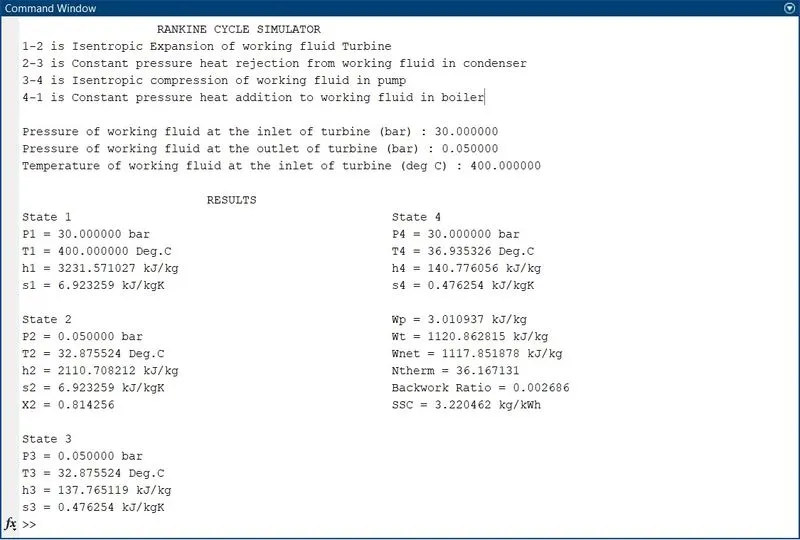
fprintf('                          RESULTS                             \n')
fprintf('State 1                                             State 4\n')
fprintf('P1 = %f bar                                  P4 = %f bar\n',p1,p4)
fprintf('T1 = %f Deg.C                               T4 = %f Deg.C\n',T1,T4)
fprintf('h1 = %f kJ/kg                              h4 = %f kJ/kg\n',h1,h4)
fprintf('s1 = %f kJ/kgK                                s4 = %f kJ/kgK\n\n',s1,s4)

fprintf('State 2                                             Wp = %f kJ/kg\n',W_P)
fprintf('P2 = %f bar                                   Wt = %f kJ/kg\n',p2,W_T)
fprintf('T2 = %f Deg.C                                Wnet = %f kJ/kg\n',T2,W_net)
fprintf('h2 = %f kJ/kg                              Ntherm = %f\n',h2,ntherm)
fprintf('s2 = %f kJ/kgK                                Backwork Ratio = %f\n',s2,Backworkratio)
fprintf('X2 = %f                                       SSC = %f kg/kWh\n\n',X2,Steamrate)

fprintf('State 3\n')
fprintf('P3 = %f bar\n',p3)
fprintf('T3 = %f Deg.C\n',T3)
fprintf('h3 = %f kJ/kg\n',h3)
fprintf('s3 = %f kJ/kgK\n',s3)
Program Logic & Stepwise explanation of code
Step 1
Given: Xteam function file, p1 – turbine inlet pressure, p2 – turbine outlet pressure & T1 – temperature at inlet of turbine.
XSteam function file is downloaded and saved in the same folder as the current program. XSteam function file contains all the properties of water and steam with valid steam table functions. The properties are as per Industrial Formulation 1997 (IF97) authorised by IAPWS.
Calculation of State 1 properties
Using the functions h_pT & s_pT from XSteam file – enthalpy as a function of pressure and temperature & entropy as a function of pressure and temperature at state 1 respectively.
h1=XSteam('h_pT',p1,T1);
s1=XSteam('s_pT',p1,T1);
Calculation of State 2 properties
Entropy is constant from state 1 to state 2 as it is an isentropic process. Therefore, s2=s1.
To determine h2, dryness fraction at state point 2 is calculated using entropy and is substituted in dryness fraction formula using enthalpy.
Dryness fraction
The steam dryness fraction is used to quantify the amount of water within steam. If steam contains 10% water by mass, it's said to be 90% dry, or have a dryness fraction of 0.9.
Steam dryness is important because it has a direct effect on the total amount of transferable energy contained within the steam (usually just latent heat), which affects heating efficiency and quality.
For example, saturated steam (100% dry) contains 100% of the latent heat available at that pressure. Saturated water, which has no latent heat and therefore 0% dryness, will only contain sensible heat.
X2=(s2-sl2)/(sg2-sl2);
h2=(hg2-hl2)*X2+hl2;
X2 – dryness fraction, sl2 – entropy of wet saturation steam, sg2 – entropy of dry saturated steam,
hl2 - enthalpy of wet saturation steam, sg2 – enthalpy of dry saturated steam,
hl2,sl2,hg2 and sg2 are functions of pressure and are determined using XSteam function with p2 as input.
T2 is a function of h and s and is determined using XSteam function with h2 an s2 as inputs
Calculation of State 3 properties
Pressure at outlet of turbine = pressure at inlet of condenser i.e., p3=p2
The heat rejection that takes place in process 2 – 3 is latent heat, therefore, temperature remains constant. i.e., T3=T2
Since the condenser outlet contains the saturated liquid or wet saturated steam,
h3 and s3 can be determined as a function of pressure using XSteam function with p3 as input.
Process 3 -4 is work done by pump Wp = ʃ Vdp = v3(p4-p3)
v3 – specific volume or volume/unitmass.
v3 is a function of pressure and determined using XSteam function with p3 as input
v3=XSteam('vL_p',p3);
Work done by pump is
W_P=v3*(p4-p3)*100; (pressure in bar is converted to kPa to obtain work in kJ/kg)
Calculation of State 4 properties
Pressure at outlet of pump = pressure at inlet of boiler i.e., p4=p1
Process 3 – 4 is an isentropic compression process, therefore, s4=s3
Determining T4 using isentropic relation between T and P from state 3 to state 4
(p4/p3)^r=T4/T3|T4 = T3(p4/p4)^r (this relation is obtained by considering that working fluid obeys ideal gas equation i.e., PV=nRT)
Let r = (ɣ-1)/ɣ; ɣ = Cp4/Cv4 at state 4.
Cp4 and Cv4 – specific heat of working fluid at constant pressure and volume at state 4.
Cp and Cv are functions of p and s and determined using XSteam function with p4 and s4 as inputs
Cp4=XSteam('Cp_ps',p4,s4);
Cv4=XSteam('Cv_ps',p4,s4);
gamma = Cp4/Cv4;
r = (gamma-1)/gamma;
T4=T3*(p4/p3)^r;
To calculate h4, using S.F.E.E. for pump
Wp = h4-h3|h4=Wp+h3 (Wp is already calculated using flow work equation)
h4=h3+W_P;
Step 2
Calculation of Thermal efficiency, Backwork ratio and SSC
Thermal efficiency is ratio net work output to heat supplied by boiler
= Wt-Wp/Q1
Wt=h1-h2; Q1=h4-h3
Backwork ratio
The backwork ratio is the fraction or percentage of work that the turbine produces that is consumed by the pump. It is the ratio of required pump work to turbine work generated.
Backwork ratio = Wp/Wt
SSC (Specific Steam Consumption or Steam Rate)
The capacity of a steam plant is often expressed in terms of steam rate, which is defined as the rate of steam flow (kg/h) required to produce unit shaft output (1kW).
Steam rate = mass of steam (kg/h)/Wnet (kW)
= m(kg/h)/m(kg/s)xWnet(kJ/kg)
= 3600/Wnet(kJ/kWh)
Step 3
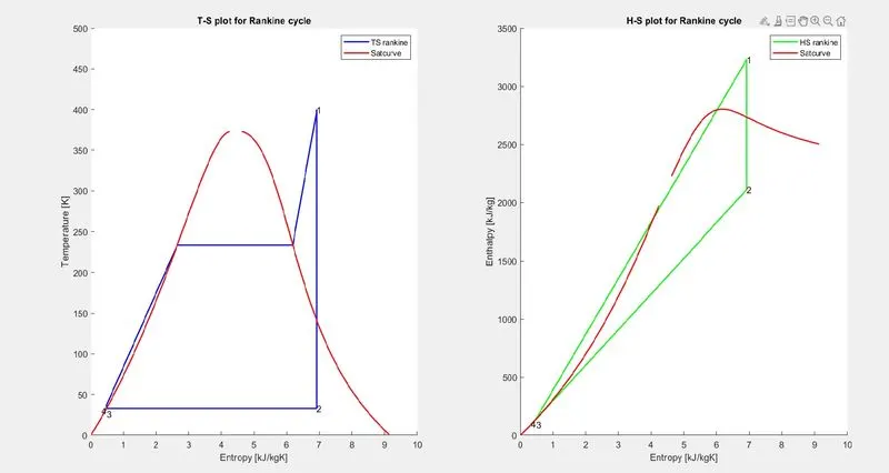
Generation of T-S and H-S plots
For accurate T-S plot , we require extra plotting points i.e, T5, T6 and s5,s6 other than state points from 1 to 4.
plot points 5 and 6 are on saturation curve, therefore, T5 is determined using T as a function of p with p1 as input and T6=T5 (latent heat of vaporisation, temperature remains constant)
s5 ans s6 are determined using s as a function of p with p1 as input.
To plot saturation curve, T_satcurve vector is generated using linspace command, the temperatures range from 1 to 500 with 500 values.
Entropy vectors are generated for wet saturated steam(sL) and dry saturated steam(sV). Entropy is taken as a function temperature with element of T_satcurve as an input. To generate entropy vectors, for loop is initiated with iterations = length of T_satcurve vector. For each element of T_satcurve vector, one element of sL vector is generated, similarly an element is generated for sV vector.
Same procedure is repeated for enthalpy vectors for wet and dry saturated steams for saturation curve of HS plot.
Generation of subplots (1,2,1) & (1,2,2)– one for TS and other for HS
[(1,2,1) – 1 row, 2 column, 1st plot, (1,2,2) – 1 row, 2 column, 2nd plot]
Plot generation of T-S diagram & saturation curve using plot function
plot([s1 s2 s3 s4 s5 s6 s1],[T1 T2 T3 T4 T5 T6 T1],'lineWidth',1.5,'color','b')
plot(sL,T_satcurve,'lineWidth',1.5,'color','r')
plot(sV,T_satcurve,'lineWidth',1.5,'color','r')
Plot generation of H-S diagram & saturation curve using plot function
plot([s1 s2 s3 s4 s1],[h1 h2 h3 h4 h1],'lineWidth',1.5,'color','g')
plot(sL,hL,'lineWidth',1.5,'color','r')
plot(sV,hV,'lineWidth',1.5,'color','r')
Step 4
Generation of data in command window or output screen
fprintf command is used to print all the data in the output screen or command window.
%f is used for floating point numbers, \n is used for new line, ‘ ‘ or single quotes are used to print the data as entered.
RESULTS
1) OUTPUT SCREEN
PLOTS
Errors
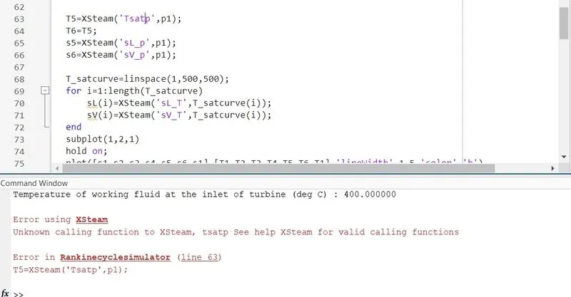
Improper typing of function - Tsatp
Correction - Tsat_p