A code in MATLAB to optimize the stalagmite function using Genetic Algorithm.
Aim:
- To write a code in MATLAB to optimise the stalagmite function and find the global maxima of the function.
- Clearly explain the concept of genetic algorithm in your own words and also explain the syntax for ga in MATLAB in your report.
- Make sure that your code gives the same output, even if it is made to run several times.
- Plot graphs for all 3 studies and for F maximum vs no. of iterations. Title and axes labels are a must, legends could be shown if necessary.
Genetic Algorithm:
Genetic algorithm solves smooth or non-smooth optimization problems with any types of constraints, including integer constraints. It is a stochastic, population-based algorithm that searches randomly by mutation and crossover among population members.
A genetic algorithm (GA) is a method for solving both constrained and unconstrained optimization problems based on a natural selection process that mimics biological evolution. The algorithm repeatedly modifies a population of individual solutions. At each step, the genetic algorithm randomly selects individuals from the current population and uses them as parents to produce the children for the next generation. Over successive generations, the population "evolves" toward an optimal solution.
You can apply the genetic algorithm to solve problems that are not well suited for standard optimization algorithms, including problems in which the objective function is discontinuous, nondifferentiable, stochastic, or highly nonlinear.
In MATLAB the Genetic Algorithm solver is abbreviated as “ga”. Which is only used to find minimum of a function.
Syntax:
x = ga(fun,nvars) finds a local unconstrained minimum, x, to the objective function, fun. nvars is the dimension (number of design variables) of fun.
x = ga(fun,nvars,A,b) finds a local minimum x to fun, subject to the linear inequalities A*x ≤ b. ga evaluates the matrix product A*x as if x is transposed (A*x').
x = ga(fun,nvars,A,b,Aeq,beq) finds a local minimum x to fun, subject to the linear equalities Aeq*x = beq and A*x ≤ b. (Set A=[] and b=[] if no linear inequalities exist.) ga evaluates the matrix product Aeq*x as if x is transposed (Aeq*x').
x = ga(fun,nvars,A,b,Aeq,beq,lb,ub) defines a set of lower and upper bounds on the design variables, x, so that a solution is found in the range lb ≤ x ≤ ub. (Set Aeq=[] and beq=[] if no linear equalities exist.)
x = ga(fun,nvars,A,b,Aeq,beq,lb,ub,nonlcon) subjects the minimization to the constraints defined in nonlcon. The function nonlcon accepts x and returns vectors C and Ceq, representing the nonlinear inequalities and equalities respectively. ga minimizes the fun such that C(x) ≤ 0 and Ceq(x) = 0. (Set lb=[] and ub=[] if no bounds exist.)
x = ga(fun,nvars,A,b,Aeq,beq,lb,ub,nonlcon,options) minimizes with the default optimization parameters replaced by values in options. (Set nonlcon=[] if no nonlinear constraints exist.) Create options using optimoptions.
x = ga(fun,nvars,A,b,[],[],lb,ub,nonlcon,IntCon) or x = ga(fun,nvars,A,b,[],[],lb,ub,nonlcon,IntCon,options) requires that the variables listed in IntCon take integer values.
x = ga(problem) finds the minimum for problem, a structure described in problem.
[x,fval] = ga(___), for any previous input arguments, also returns fval, the value of the fitness function at x.
[x,fval,exitflag,output] = ga(___) also returns exitflag, an integer identifying the reason the algorithm terminated, and output, a structure that contains output from each generation and other information about the performance of the algorithm.
[x,fval,exitflag,output,population,scores] = ga(___) also returns a matrix population, whose rows are the final population, and a vector scores, the scores of the final population.
Stalagmite Function to be optimized:
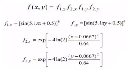
Stalagmite Function Code:
function [F] = stalagmite_function(input_vector)

x = input_vector(1);
y = input_vector(2);

f1x = (sin(5.1*pi*x + 0.5)).^6 ;
f1y = (sin(5.1*pi*y + 0.5)).^6 ;

f2x = exp (-4 * log(2) * (((x - 0.0667).^2)/0.64)) ;
f2y = exp (-4 * log(2) * (((y - 0.0667).^2)/0.64)) ;

F = -(f1x * f1y * f2x * f2y) ;

end
Stalagmite Function Code with explanation:
% Firstly we will write our fitness function:
% here we have two input argument a & b.
function [F] = stalagmite_function(input_vector)
x = input_vector(1);
y = input_vector(2);
f1x = (sin(5.1*pi*x + 0.5)).^6 ;
f1y = (sin(5.1*pi*y + 0.5)).^6 ;
f2x = exp (-4 * log(2) * (((x - 0.0667).^2)/0.64)) ;
f2y = exp (-4 * log(2) * (((y - 0.0667).^2)/0.64)) ;
F = -(f1x * f1y * f2x * f2y) ;
%since Genetic algotitm only minimises the function, in order to maximise it we put a negative sign.
end
Programme Code:
close all
clear all
clc


x = linspace (0,0.6,150);
y = linspace (0,0.6,150);


[X,Y] = meshgrid(x,y);


for i = 1:length(X)
    for j = 1:length(Y)
        input_vector(1) = X(i,j);
        input_vector(2) = Y(i,j);
        F(i,j) = stalagmite_function(input_vector);
    end
end


figure(1)
surfc(X,Y,-F)
xlabel('x-values')
ylabel('y-values')
zlabel('F-value')
shading interp


% Study 1: Statistical Behaviour

iteration = 50;

tic
for i = 1 : iteration
    [input, Fopt(i)] = ga(@stalagmite_function,2);
     xopt(i) = input(1);
     yopt(i) = input(2);
end


study1_time = toc;

figure(2)
subplot(2,1,1)
surfc(X,Y,-F)
xlabel('x')
ylabel('y')
shading interp

hold on


plot3(xopt,yopt,-Fopt,'color','b', 'marker','o','markersize',5,'markerfacecolor','r');
title('Case-1: Unbounded inputs')

subplot(2,1,2)
plot(-Fopt)
xlabel('Iteration')
ylabel('Function maximum value')


% Case 2 / Statistical behaviour with upper and Lower bounds

tic
for i = 1 : iteration
    [input2,Fopt(i)] = ga(@stalagmite_function,2, [],[],[],[],[0;0],[0.4;0.4]);
    xopt(i) = input2(1);
    yopt(i) = input2(2);
end

study_2_time = toc;

figure(3)

subplot(2,1,1)
surfc(X,Y,-F);
xlabel('x')
ylabel('y')
shading interp

hold on

plot3(xopt,yopt,-Fopt,'marker','o','markersize',5,'markerfacecolor','r')
title('Case-2: Bounded inputs')

subplot(2,1,2)
plot(-Fopt)
xlabel('Iteration')
ylabel('Function maximum value')

% Case 3 : Now in addition to specifying the bounds.


options = optimoptions('ga');
options = optimoptions(options, 'PopulationSize',100);

tic
for i = 1 : iteration
    [input3, Fopt(i)] = ga(@stalagmite_function,2,[],[],[],[],[0;0],[0.4;0.4],[],[],options);
    xopt(i) = input3(1);
    yopt(i) = input3(2);
end


study_3_time = toc;

figure(4)
subplot(2,1,1)

surfc(X,Y,-F)
shading interp
xlabel('x')
ylabel('y')

hold on

plot3(xopt,yopt,-Fopt,'marker','o','markersize',5,'markerfacecolor','r');
title('Case-3: Bounded inputs with increased polpulation size')
subplot(2,1,2)
plot(-Fopt)
xlabel('Iteration')
ylabel('Function maximum value')
Programme Code with explanation:
close all
clear all
clc
%Input arrays for GA, this does not define the search space for GA, since GA does not know this is our search space.
x = linspace (0,0.6,150);
y = linspace (0,0.6,150);
[X,Y] = meshgrid(x,y);
% Evaluating the stalagemite function.
% "for" command is used for loop operation.
% "input vector" store the value of matrix 'X' & 'Y'
% "input vector" goes to "stalagmite_function" and after being evaluated, output
% is stored in matrix 'F'.
for i = 1:length(X)
for j = 1:length(Y)
input_vector(1) = X(i,j);
input_vector(2) = Y(i,j);
F(i,j) = stalagmite_function(input_vector); % Calling the function.
end
end
%"surfc" command creats a 3D surface plot with contour underneath. The 'X' & 'Y' are
% ploted in x-axis and y-axis. Evaluated Function values stored in matrix 'F' are ploted
% in Z-axis, giving the plot a 3D look.
% "shading interp" is used to hide the grid line on the plot.
figure(1)
surfc(X,Y,-F)
xlabel('x-values')
ylabel('y-values')
zlabel('F-value')
shading interp
% Case 1: Statistical Behaviour.
iteration = 50; % It defines number of iteration in the algorithm.
% "tic-toc" command is used to calculate the time of running command.
% [x,fval] = ga(___), it finds the minimum for problem and also returns 'fval', the value of the fitness function at x.
tic
for i = 1 : iteration
[input, Fopt(i)] = ga(@stalagmite_function,2);
xopt(i) = input(1);
yopt(i) = input(2);
end
study1_time = toc;
% Plotting the Graph
figure(2)
subplot(2,1,1)
surfc(X,Y,-F)
xlabel('x')
ylabel('y')
shading interp
hold on
% using plot3 command to plot x, y and optimum function value that GA pridicts over 50 studies.
plot3(xopt,yopt,-Fopt,'color','b', 'marker','o','markersize',5,'markerfacecolor','r');
title('Case-1: Unbounded inputs')
subplot(2,1,2)
plot(-Fopt) %Ploting optimum value the function is pridicting over 50 iteration.
xlabel('Iteration')
ylabel('Function maximum value')
% Case 2: Statistical behaviour with upper and Lower bounds.
tic
for i = 1 : iteration
[input2,Fopt(i)] = ga(@stalagmite_function,2, [],[],[],[],[0;0],[0.4;0.4]);
xopt(i) = input2(1);
yopt(i) = input2(2);
end
study_2_time = toc;
%Ploting Graph
figure(3)
subplot(2,1,1)
surfc(X,Y,-F);
xlabel('x')
ylabel('y')
shading interp
hold on
plot3(xopt,yopt,-Fopt,'marker','o','markersize',5,'markerfacecolor','r')
title('Case-2: Bounded inputs')
subplot(2,1,2)
plot(-Fopt)
xlabel('Iteration')
ylabel('Function maximum value')
% Case 3 : Now in addition to specifying the bounds, we are going to change initial population size. Because if the sample size is too small it may not find global minima but local minima. Only drawback is it willslowdown GA bec of more sample.
options = optimoptions('ga');
options = optimoptions(options, 'PopulationSize',100);
tic
for i = 1 : iteration
[input3, Fopt(i)] = ga(@stalagmite_function,2,[],[],[],[],[0;0],[0.4;0.4],[],[],options);
xopt(i) = input3(1);
yopt(i) = input3(2);
end
study_3_time = toc;
%Ploting Graph
figure(4)
subplot(2,1,1)
surfc(X,Y,-F)
shading interp
xlabel('x')
ylabel('y')
hold on
plot3(xopt,yopt,-Fopt,'marker','o','markersize',5,'markerfacecolor','r');
title('Case-3: Bounded inputs with increased polpulation size')
subplot(2,1,2)
plot(-Fopt)
xlabel('Iteration')
ylabel('Function maximum value')
Conclusion:
Case 1:
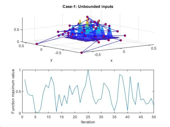
The result shows, maxima vary over a large size of interval, providing vague idea of global maxima. Through particular value of global maxima can’t be determined but by observation it can be figured that the value of global maximum lies b/w the interval [0,1].
Study time for this case was the least of all the three i.e 4.7438 seconds.
Case 2:
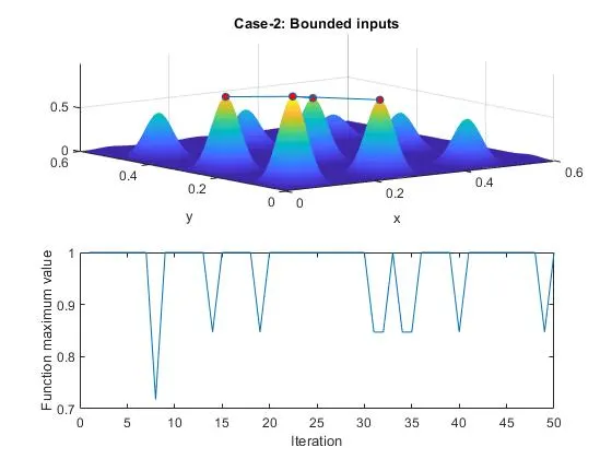
Through guess we have defined the bounds hence we could only get the values within our range. After providing the boundary limits the variation in in the optimum values have reduced. Form the plot it can be infer that the global maxima lie in the range [0.85,1].
The study took 6.3140 seconds.
Case 3:
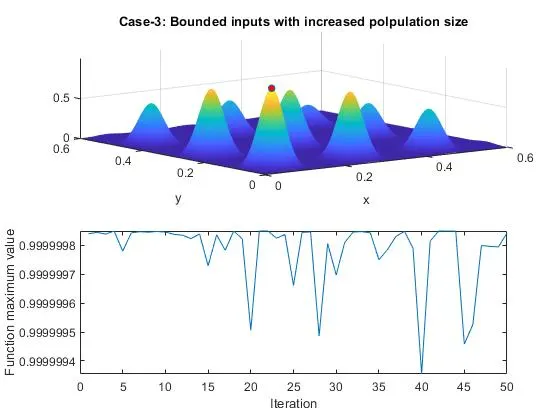
By increasing the population size and incorporating bounded inputs, we have more probability of determining the Global maxima. Since the number of iterations have increased the took longer than the previous two to execute, it took 10.96289 seconds. Global maximum is 0.9999998.