A MATLAB code to solve Air-standard Otto cycle problems by providing values of Pressure, Volume, Temperature & Thermal Efficiency and to make it's P-V plot.
1) Code to solve Air-standard otto cycle problems and to make it's P-V plot.
clear all
close all
clc

% Inputs Given :-
% Pressure and Temperature at the beginning of the compression stroke are 1bar and 27deg C.
% p1 = 1 bar = 1 * 10^(5) N/m^2
% p3 = 30 bar
% T1 = 27 deg C = 300K

% Engine Geometric parameters
% r = compression ration
% Unit of length = meter, Temperature = Kelvin, pressure = N/m^2 & Volume= m^3.

gamma = 1.4;
bore = 0.1;
stroke = 0.1;
con_rod = 0.15;
r = 5.5;

% Calculating the swept volume and the clearance voume.
% r = Total volume(v1) / clearance volume = (v_swept + v_clearance) / v_clearance
v_swept = (pi/4)*bore^2 * stroke;
v_clearance = v_swept / (r - 1);

v1 = v_swept + v_clearance;
v2 = v_clearance;
v3 = v2;
v4 = v1;

% Calculating Pressure
% using pv^(gamma) = constant    and   r = v1/v2
% p4 = p3 * (v3/v4)^(gamma) = p3 * (1/r)^(gamma)
p1 = 1 * 10^5;
p2 = p1 * r^(gamma);
p3 = 30 * 10^5;
p4 =  p3 * (1/r)^(gamma);

% Calculating Temperature
% using,  p1 * v1 / T1 = p2 * v2 / T2    =>  T2 / T1 = r ^(gamma-1)
T1 = 300;
T2 = T1 * r ^(gamma-1);
T3 = T2 * (p3 / p2);
T4 = T1 * (p4 / p1);

% Calculating Pressure and volume at every point during compression by calling a function
constant_c1 = p1*v1^gamma;

V_compression = Piston_Kinematics_function(bore,stroke,con_rod,r,180,0);

P_compression = constant_c1 ./ V_compression.^gamma;

% Calculating Pressure and volume at every point during expansion by calling a function
constant_c2 = p3*v3^gamma;

V_expansion = Piston_Kinematics_function(bore,stroke,con_rod,r,0,180);

P_expansion = constant_c2 ./ V_expansion.^gamma;

% Calculating thermal effeciency

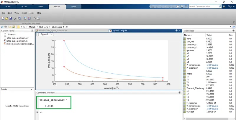
Thermal_Effeciency = 1 - (1 / r^(gamma-1))


% Convrting pressure unit from N/m^2 to "bar"
p1 = 10^(-5) * p1;
p2 = 10^(-5) * p2;
p3 = 10^(-5) * p3;
p4 = 10^(-5) * p4;
P_compression = 10^(-5) * P_compression;
P_expansion = 10^(-5) * P_expansion;

% Changing m^3 to cm^3
v1 = 10^6 * v1;
v2 = 10^6 * v2;
v3 = 10^6 * v3;
v4 = 10^6 * v4;
V_compression = 10^6 * V_compression;
V_expansion = 10^6 * V_expansion;


% Plotting


figure(1)
hold on
plot(v1,p1,'*','color','r')
plot(V_compression, P_compression)
plot(v2,p2,'*','color','r')
plot([v2 v3],[p2 p3])
plot(v3,p3,'*','color','r')
plot(V_expansion, P_expansion)
plot(v4,p4,'*','color','r')
plot([v1 v4],[p1 p4])

xlabel('volume(cm^3)')
ylabel('pressure(bar)')
2) Function Code
function [V] = Piston_Kinematics_function(bore, stroke, con_rod, r, start_crank, end_crank)

% This function provides the value of volume at every point while the piston compresses and expands.

% Engine Geometric parameters
% r = compression ration

a = stroke/2;
R = con_rod/a;

% Calculating the swept volume and the clearance voume.
% r = Total volume(v1) / clearance volume = (v_swept + v_clearance) / v_clearance
v_swept = (pi/4)*bore^2 * stroke;
v_clearance = v_swept / (r - 1);

theta = linspace(start_crank,end_crank,100);

term1 = 0.5 * (r-1);
term2 = R+1-cosd(theta);
term3 = (R^2 - sind(theta).^2).^0.5;

V = (1 + term1 * (term2 - term3)).* v_clearance;

end
3) Output
4) Report
Defining the terms used :
Bore = Nominal inner diameter of the cylinder.
Stroke = Nominsal distance travelled by the piston between 2 successive reversal in its direction of motion.
Swept voulme = nominal volume swept by the piston as it travell from Top dead center(TDC) to Bottom dead center(BDC).
Clearance volume = Nominal volume of the combustion chamber when the piston is at TDC.
Compression Ratio(r) = ratio of cylinder volume at BDC to the clerance volume.
Gamma = Ratio of specific heats (Cp/Cv) for air. It is 1.4 air.
Explaning the code stepwise:-
<<>>
%Providing inputs to the programme. Which will help in calculating other dependent variables.
% p1 = 1 bar = 1 * 10^(5) N/m^2
% p3 = 30 bar
% T1 = 27 deg C = 300K
gamma = 1.4;
bore = 0.1;
stroke = 0.1;
con_rod = 0.15;
r = 5.5;
<<>>
%Calculating dependent variable using input values.
%Formulaes used :-
v_swept = (pi/4)*bore^2 * stroke;
v_clearance = v_swept / (r - 1);
v1 = v_swept + v_clearance
v2 = v_clearance
v3 = v2
v4 = v1
% Calculating Pressure
% using pv^(gamma) = constant and r = v1/v2
% p4 = p3 * (v3/v4)^(gamma) = p3 * (1/r)^(gamma)
p1 = 1 * 10^5
p2 = p1 * r^(gamma)
p3 = 30 * 10^5
p4 = p3 * (1/r)^(gamma)
% Calculating Temperature
% using, p1 * v1 / T1 = p2 * v2 / T2 => T2 / T1 = r ^(gamma-1)
T1 = 300
T2 = T1 * r ^(gamma-1)
T3 = T2 * (p3 / p2)
T4 = T1 * (p4 / p1)
Thermal_Effeciency = 1 - (1 / r^(gamma-1))
<<>>
% Calculating Pressure and volume at every point during compression and expansion by calling a function.
% We have already saved an appropriate function in another file and we are using the below mention command to call the function
% and calculate the values for pressure and volume at every point during compression and expansion phase.
constant_c1 = p1*v1^gamma;
V_compression = Piston_Kinematics_function(bore,stroke,con_rod,r,180,0);
P_compression = constant_c1 ./ V_compression.^gamma;
constant_c2 = p3*v3^gamma;
V_expansion = Piston_Kinematics_function(bore,stroke,con_rod,r,0,180);
P_expansion = constant_c2 ./ V_expansion.^gamma;
<<>>
% For convinence we are converting pressure unit to "bar" and Volume to "cm^3".
% Convrting pressure unit from N/m^2 to "bar"
p1 = 10^(-5) * p1
p2 = 10^(-5) * p2
p3 = 10^(-5) * p3
p4 = 10^(-5) * p4
P_compression = 10^(-5) * P_compression
P_expansion = 10^(-5) * P_expansion
% Changing m^3 to cm^3
v1 = 10^6 * v1
v2 = 10^6 * v2
v3 = 10^6 * v3
v4 = 10^6 * v4
V_compression = 10^6 * V_compression
V_expansion = 10^6 * V_expansion
<<>>
% Plotting
% Now, we are plotting P-V diagram.
% Command "plot(vn,pn,'*','color','r')" is used to plot v1, v2, v3, v4, p1, p2, p3 & p4.
% Command "plot(V_compression, P_compression)" is used to plot every point during compression when the crank move 180deg to 0deg.
% Similarly "plot(V_expansion, P_expansion)" command is used.
% Finally, command "plot([v2 v3],[p2 p3]) & plot([v1 v4],[p1 p4])" are used to draw a straight line.
figure(1)
hold on
plot(v1,p1,'*','color','r')
plot(V_compression, P_compression)
plot(v2,p2,'*','color','r')
plot([v2 v3],[p2 p3])
plot(v3,p3,'*','color','r')
plot(V_expansion, P_expansion)
plot(v4,p4,'*','color','r')
plot([v1 v4],[p1 p4])
% Below mentioned commands are used to mention label names in x and y-axis.
xlabel('volume(cm^3)')
ylabel('pressure(bar)')
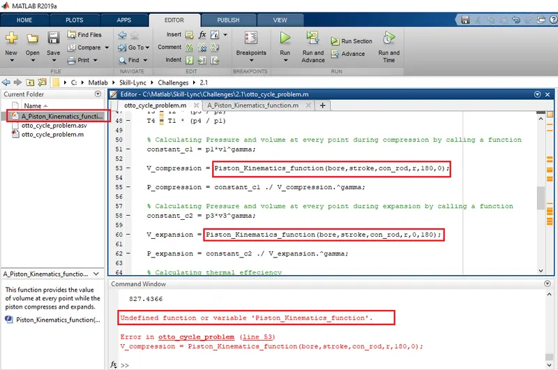
ERROR faced :
My Function name and Function file name were different, so when i called the function while running the final program
Matlab showed an error "Undefined function or variable".
Rectifying the ERROR :
I make sure the function name and function file name to be the same.
Error Screenshot