Generic algorithm program for optimization of values of a given function using MATLAB.

Aim – To calculate the generic algorithm for calculating the local maxima and calculating the optimum values for a given function.

Introduction – Generic algorithm uses the method of random sampling. This method of solving constrained and unconstrained problems which are based upon selection. Generic algorithm is widely used to solve the optimization problems in different fields.

Generic algorithm starts with an initial set of random solutions called population.

Each individual in the population is called chromosome representing a solution to the problem at hand.

The chromosome evolves through the successive iterations, called generations.

During each generation, the chromosomes are evaluated using some measures of fitness.

To create a new generation, new chromosome are formed by either merging two chromosomes from current generation using a crossover operator or modifying a chromosome using mutation operator.

A new generation is formed by selecting according to fitness values and rejecting others so as to keep the population size constant.

Stalagmite function is the mathematical model for generating the local minima and maxima.

Code for the generic algorithm of a stalagmite function –

%ga case 1 - Unbounded Inputs
clear all
close all
clc

x = linspace(0,0.6,150);
y = linspace(0,0.6,150);
n_var = 100;
[xx, yy] = meshgrid(x,y);
for i = 1:length(xx)
    for j = 1:length(yy)
        input_vector(1) = xx(i,j);
        input_vector(2) = yy(i,j);
        f(i,j) = stalagmite_basic(input_vector);
    end
end

tic
for i = 1:n_var
    [input,fopt(i)] = ga(@stalagmite_basic,2);
        xopt(i) = input(1);
        yopt(i) = input(2);
end
studytime_case1 = toc

figure(1)
subplot(2,1,1)
surfc(x,y,f)
shading interp
hold on
plot3(xopt,yopt,fopt,'marker','o','markersize',5,'markerfacecolor','r')
subplot(2,1,2)
plot(fopt)
title('Unbounded Inputs');
xlabel('Iterations');
ylabel('Function minimum');

%Study case 2- Bounded inputs.
tic
for i = 1:n_var
    [input,fopt(i)] = ga(@stalagmite_basic,2,[],[],[],[],[0;0],[1;1]);
        xopt(i) = input(1);
        yopt(i) = input(2);
end
studytime_case2 = toc

figure(2)
subplot(2,1,1)
surfc(x,y,f)
shading interp
hold on
plot3(xopt,yopt,fopt,'marker','o','markersize',5,'markerfacecolor','r')
subplot(2,1,2)
plot(fopt)
title('Bounded Inputs');
xlabel('Iterations');
ylabel('Function minimum');

%Study case 3- Bounded Inputs with Popolation size

options = optimoptions('ga');
options = optimoptions(options,'PopulationSize',500);

tic
for i = 1:n_var
    [input,fopt(i)] = ga(@stalagmite_basic,2,[],[],[],[],[0;0],[1;1],[],[],options);
        xopt(i) = input(1);
        yopt(i) = input(2);
end
studytime_case3 = toc
figure(3)
subplot(2,1,1)
surfc(x,y,f)
shading interp
hold on
plot3(xopt,yopt,fopt,'marker','o','markersize',5,'markerfacecolor','r')
subplot(2,1,2)
plot(fopt)
title('Bounded Inputs with Population Size');
xlabel('Iterations');
ylabel('Function minimum');

Explanation –

The values of x and y are given from 0 to 0.6 with 150 intervals between them. Plot is converted into 2D by meshgrid command. Three cases has been done in this problem.

In first case, n_var is the number of iterations as 100. So genetic algorithm will be run 100 times and will find the optimum values. In order to implement the generic algorithm syntax, first for loop is used for the calculation of z surface values from the given function with all values of x and y. Then generic algorithm syntax is used with for loop for 100 iterations. First case is an unbounded input case with no input constraints. Hence, in ga syntax only calculated stalagmite function and input variables are given and outputs obtained are the optimum values of x, y and function optimum values for given x and y.

tic-toc command is used to calculate the time required for ga syntax to implement the code. Surface command is used to plot the surface and shading interp command smoothen the curve. With the help of subplots, 2 plots are plotted in which, one is to plot the optimum values of x,y and f & second is used to describe the optimum values of f for given x and y.

In second case, to reduce the optimum values and ultimately to reduce the complexity of the plot, constraints are given in the form of boundary conditions. So that the ga loop changes with adding the co-ordinates (i.e. boundary conditions) as 0,0 and 1,1. Four square brackets describe no equality and inequality constraints.

Still the obtained plot has many optimum values. Thus more constraint is given by increasing the population size to 500 in the third case. Optimoptions is the function by which parameters in ga can be varied. Options is an array that is used in the ga syntax, particularly used to save the optimoptions (i.e. altered parameters of ga).

Generic Algorithm Syntax –

For case 1:

[input,fopt(i)] = ga(@stalagmite_basic,2);

Input = inputs or co-ordinates

fopt(i) = Optimum values found out by ga in iteration i.

ga = function to implement generic algorithm.

stalagmite_basic = given calculated stalagmite function called in the main program.

2 = No. of variables.

For case 2:

[input,fopt(i)] = ga(@stalagmite_basic,2,[],[],[],[],[0;0],[1;1])

Input = inputs or co-ordinates

fopt(i) = Optimum values found out by ga in iteration i.

ga = function to implement generic algorithm.

stalagmite_basic = given calculated stalagmite function called in the main program.

2 = No. of variables.

[],[] = First two brackets describe the linear inequality constrains with the conditions that should be fulfilled by the ga syntax. (Due to not having any values there are no such conditions in the problem.)

[],[] = Last two brackets describe the linear equality constrains with the conditions that should be fulfilled by the ga syntax. (Due to not having any values there are no such conditions in the problem.)

[0;0] = Lower boundary (i.e. co-ordinates) of the equation.

[1;1] = Upper boundary (i.e co-ordinates) of the equation.

For case 3:

[input,fopt(i)] = ga(@stalagmite_basic,2,[],[],[],[],[0;0],[1;1],[],[],options)

Input = inputs or co-ordinates

fopt(i) = Optimum values found out by ga in iteration i.

ga = function to implement generic algorithm.

stalagmite_basic = given calculated stalagmite function called in the main program.

2 = No. of variables.

[],[] = First two brackets describe the linear inequality constrains with the conditions that should be fulfilled by the ga syntax. (Due to not having any values there are no such conditions in the problem.)

[],[] = Next two brackets describe the linear equality constrains with the conditions that should be fulfilled by the ga syntax. (Due to not having any values there are no such conditions in the problem.)

[0;0] = Lower boundary (i.e. co-ordinates) of the equation.

[1;1] = Upper boundary (i.e co-ordinates) of the equation.

[],[] = Last two brackets represent the non-linear inequality constraints with the conditions that should be fulfill by the ga syntax. (Due to not having any values there are no such conditions in the problem.)

options = options is used to implement the altered parameters of ga in the main program.

Code for the stalagmite function –

function [Z] = stalagmite_basic(input_vector)
x = input_vector(1);
y = input_vector(2);


f1x = (sin(5.1*pi.*x + 0.5)).^6;
f1y = (sin(5.1*pi.*y + 0.5)).^6;

f2x = exp(-4*log(2).*((x-0.0667).^2/(0.64)));
f2y = exp(-4*log(2).*((y-0.0667).^2/(0.64)));

fx = -f1x.*f2x;
fy = f1y.*f2y;
[Z] = (fx.*fy);
end

Maxima is a function to represent the change of values from positive to negative. Hence, to find out the maxima of a given function, one of the value in the function is taken as negative. So that negative values of function minimum are obtained and the maxima can be determined. (i.e. Maxima = -Minima). In the function, values of surface z is calculated at the given values of x and y by the calculation from a given problem description. And then the optimum values has been found out in the generic algorithm program.

Results –

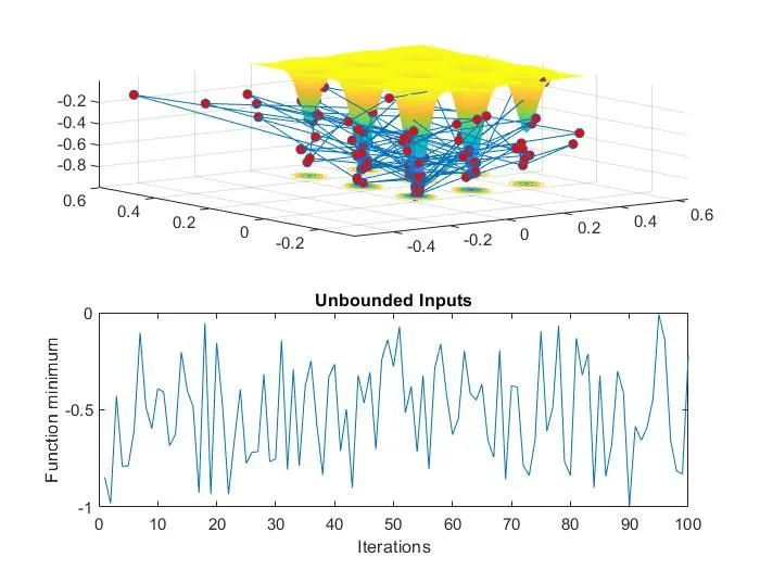
Case 1 –

The results of plot 1 is as shown below. Due to having unbounded inputs, multiple optimum values for the given stalagmite function obtained and values of given function are between 0 to -1 (i.e. Negative because of Maxima). It is very hard to find out the optimum values of a stalagmite function due to complexity of the plot. (i.e. not having the constraints.). Multiple values of maxima are obtained due to not having the constraints, which are very hard to find out from the obtained plot. The time required for ga to perform 100 iterations is 4.3592 seconds.

Case 2 –

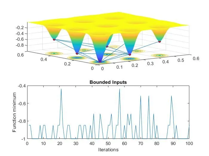
The results of Case 2 gives much more smoother plot of optimum values as compare to plot of case 1. By giving lower and upper boundary conditions, the optimum values obtained are between lower and upper bounds, which eliminates the extra optimum values and complexity of the plot. Optimum values of a given function are between -0.4 to -1 by giving the boundary conditions. Still more no of maxima obtained approximately as -0.42 for a given stalagmite function. The time required for ga to perform 100 iterations is 5.1954 seconds.

Case 3 –

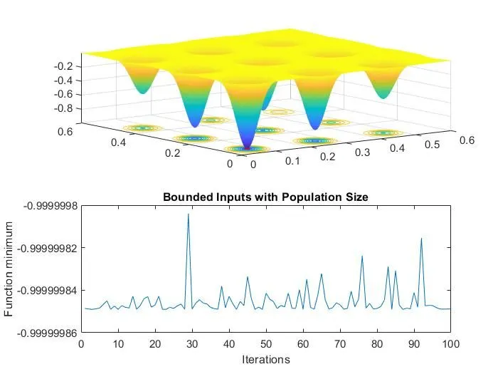
In order to get a more accurate plot, more constraints are added by giving population size to a given problem. By giving the population size, only one maxima value is obtained. So to get more accurate results, a educated guesses should be made about the constraints and less optimum results of maxima should be obtained by adding such constraints. Optimum values of a given function are between -0.99999980 to -0.99999986 by giving the population size and it reduced the no of maxima as approximately -0.99999980. The time required for ga to perform 100 iterations with population size of 500 is 34.3733 seconds. With such a high population size, calculation time increases but only one optimum value is obtained.