Curve fitting using MATLAB

Aim – To study and understand the change of mathematical data and predict the mathematical data using mathematical operations, which might not be possible in initial data set.

Introduction – Curve fitting is the process, in which curve is constructed on the basis of predictions, which possess the closest proximity to the real series of data. By curve fitting, the functional relationship between observed dataset and parameter values can be made, particularly effective to mathematically model some natural processes.

Prediction of the curve is done by nth order polynomial equation or quadratic equation or cubic function, which is solved on the basis of real data and then data is predicted mathematically by solving this equations in MATLAB. Accuracy of the predicted curve depends upon the degree of polynomials.

Initially in this project, data of Temperature and Specific heat is taken and prediction of specific heat data is found out cubically (i.e. suitable polynomial degree more than 1) and linearly (i.e. polynomial degree 1-linear regression) with the MATLAB.

Errors in Curve fitting –

Goodness of fit depends upon the errors in curve fitting, errors are as follows.

1. The sum of square due to error (SSE)
2. R- Square
3. Adjusted R-Square
4. Root mean square error

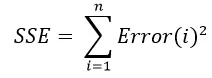
1. The sum of square due to error (SSE) – The error is found out by

2. R-Square –

R square is the square of correlation between response values and predicted response values. R- Square ranges from 0 to 1, with 0 is the worst possible fit for the data set and 1 is the best possible fit for the data set.

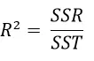
R- Square is calculated by the formula,

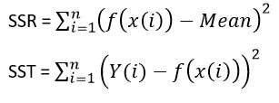
Where,

3. Adjusted R-Square –

Adjusted R-Square is a normalizing variation of R-Square which neglects the R-square due to insignificant independent variables.

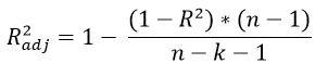
Where,

n = no of datapoints,

k = no of independent variables.

4. Root Mean Square Error –

This is known as fit standard error and the standard error for regression. It estimates the standard deviation of the data.

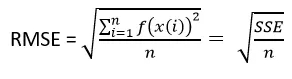
Code for Curve Fitting of given data –

% Curve fitting program
clear all
close all
clc

%Load the data
ct = load('data');
temperature = ct(:,1);
cp_actual = ct(:,2);

% curve fitting with quadratic equation = aT^3 + bT^2 + cT + d 
co_ordinates = polyfit(temperature,cp_actual,3);
cp_predicted = polyval(co_ordinates,temperature);

% plot
plot(temperature,cp_actual,'Linewidth',2, 'color', 'r');
hold on
plot(temperature, cp_predicted, 'linewidth',2,'color','b')

%Linear regression
co_ordinates_linear = polyfit(temperature,cp_actual,1);
cp_linear = polyval(co_ordinates_linear,temperature);
plot(temperature,cp_linear,'linewidth',2,'color','g');
legend('actual ct','predicted ct','linear ct')
xlabel('Temperature in K');
ylabel('specific heat in Kg/Kmol-K');
grid on

%Errors in curve fitting - cubic
error_cubic = cp_actual - cp_predicted;
SSE_cubic = sum(error_cubic.^2);
SSR_cubic = sum(cp_predicted - mean(cp_predicted)).^2;
SST_cubic = SSR_cubic + SSE_cubic;
R_square_cubic = SSR_cubic/SST_cubic;
R_mean_square_cubic = sqrt(SSE_cubic/3200);
error_cubic_percent = ((cp_actual - cp_predicted)./cp_actual)*100;
fprintf('The value of cubic error percentage is');
disp(max(error_cubic_percent))

%Errors in curve fitting - linear
error_linear = cp_actual - cp_linear;
SSE_linear = sum(error_linear.^2);
SSR_linear = sum(cp_linear - mean(cp_linear)).^2;
SST_linear = SSR_linear + SSE_linear;
R_square_linear = SSR_linear/SST_linear;
R_mean_square_linear = sqrt(SSE_linear/3200);
error_linear_percent = ((cp_actual - cp_linear)./cp_actual)*100;
y = fprintf('The value of linear error percentage is');
disp(max(error_linear_percent))

Explanation –

The mathematical data file is loaded to the workspace by the load command & the coordinates are assigned to the loaded data.

Data of specific data predicted mathematically with the equation

Where T = Temperature (i.e. independent variable on the basis of which constants a, b and c are calculated.

Degree of the polynomial equation should be kept as maximum as possible to get the correct predictions of mathematical data, but the polynomial should not be badly conditioned.

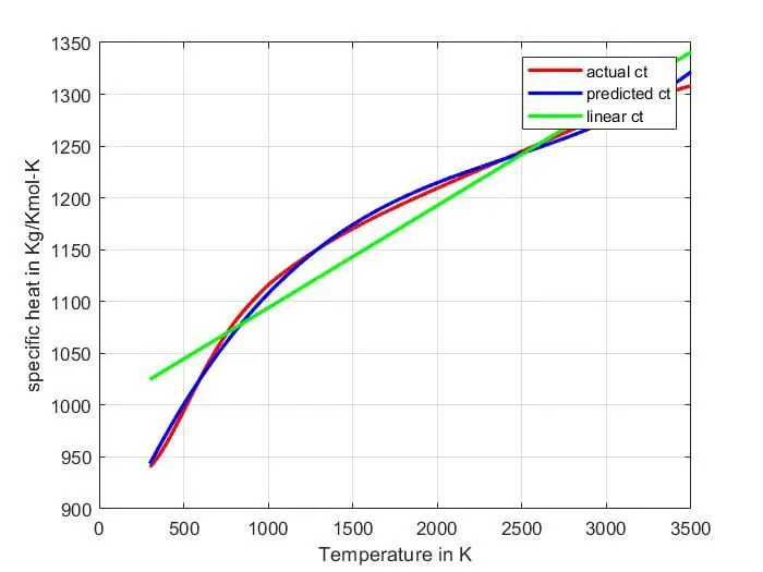
Constants a, b and c are found out by the polyfit command in the matlab, which takes the given data to find the constants. 3 is the degree of polynomial requires to implement the polyfit syntax. After finding the constants, specific heat data is predicted with the polyval command in matlab. Then given temperature vs actual data and predicted specific heat data is plotted. For linear regression degree of polynomial is given as 1 and same polyfit and polyval command is implemented and the line is plotted.

With the formulas mentioned in the introduction, different errors are calculated for cubic and linear regression and error percentage is calculated by the formula,

Results –

Figure - Temperature vs. Actual Specific heat data, Predicted cubic specific heat data and linearly predicted specific heat data.

Error calculations –

1. For cubic polynomial function,

SSE = 9.427202052073379e+04

R-Square error = 4.141303903757246e-25

Root mean square cubic error = 5.427707288784953

Max Error percent for cubic function = 0.8865%

2. For linear polynomial function,

SSE = 2.163049089179785e+06

R-Square error = 4.276561514596274e-27

Root mean square linear error = 25.999093068195336

Max Error percent for linear function = 2.4188%

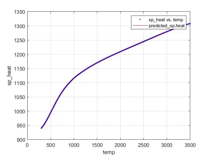
Curve Fitting by using Curve fitting toolbox in MATLAB with smoothing spline function –

Smoothing splines are smooth piecewise polynomials that can be used to represent functions over large intervals but it is impractical to load single approximate polynomial. Noisy data can be smoothly fit by smoothing spline function.

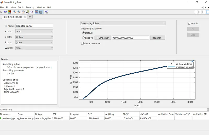
Inputs of x and y are given and smoothing spline option is selected, which gives the best possible fit with R-square =1. From this toolbox, the function is generated by generate code function.

Generated Function from smoothing spline-

function [fitresult, gof] = smoothing_spline_basictry_func(temp, sp_heat)
%CREATEFIT(TEMP,SP_HEAT)
%  Create a fit.
%
%  Data for 'predicted_sp.heat' fit:
%      X Input : temp
%      Y Output: sp_heat
%  Output:
%      fitresult : a fit object representing the fit.
%      gof : structure with goodness-of fit info.
%
%  See also FIT, CFIT, SFIT.

%  Auto-generated by MATLAB on 12-Feb-2021 13:34:34


%% Fit: 'predicted_sp.heat'.
[xData, yData] = prepareCurveData( temp, sp_heat );

% Set up fittype and options.
ft = fittype( 'smoothingspline' );

% Fit model to data.
[fitresult, gof] = fit( xData, yData, ft );

% Plot fit with data.
figure( 'Name', 'predicted_sp.heat' );
h = plot( fitresult, xData, yData );
legend( h, 'sp_heat vs. temp', 'predicted_sp.heat', 'Location', 'NorthEast', 'Interpreter', 'none' );
% Label axes
xlabel( 'temp', 'Interpreter', 'none' );
ylabel( 'sp_heat', 'Interpreter', 'none' );
grid on
end

Code to implement the smoothing spline –

clear all
close all 
clc

load('data')
temp = data(:,1);
sp_heat = data(:,2);
smoothing_function = smoothing_spline_basictry_func(temp, sp_heat)

The code is generated using this auto generated function and the plot is the best fit plot is as follows.