Generation of Pressure-Volume Diagram and Solving the Efficiency of Otto Cycle and Diesel Cycle using MATLAB.
Aim – To generate the code for plotting Pressure-Volume diagram of Otto cycle and Diesel cycle and to investigate the thermal efficiency of Otto cycle and Diesel cycle.
Introduction – Thermodynamic cycles consist of different thermodynamic processes based on some assumptions. Two thermodynamic cycles are as follows.
- Otto Cycle
- Diesel Cycle
- Otto Cycle –
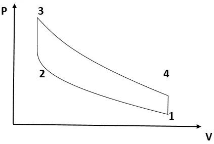
Otto cycle is also called constant volume cycle, in which two processes are isochoric processes.
Where,
Process 1-2 – Isentropic compression
Process 2-3 – Isochoric Heat Addition
Process 3-4 – Isentropic Expansion
Process 4-1 – Isochoric Heat Rejection
Code to generate Pressure-Volume diagram of Otto cycle –
%Otto Cycle Calculations(air std cycle)

%Inputs
gamma= 1.4;

%State Variables
P1 = 101325
T1 = 500
T3 = 2300

%Engine Geometry Parameters
bore = 0.1;
stroke = 0.1;
Connecting_rod = 0.15;
comp_ratio = 12;

%Calculations of Swept Volume and Clearance Volume
Vswe = (pi/4)*bore^2*stroke
Vcle = Vswe/(comp_ratio-1)

%State variables at pt1
V1 = Vswe + Vcle
V2 = Vcle

%State variables at pt 2
%Calculate P2 by P1V1^gamma = P2V2^gamma; P2 = P1V1^gamma/V2^gamma
P2 = P1*(V1/V2)^gamma

%Calculate T2 by PV/T = const; P1V1/T1 = P2V2/T2
T2 = P2*V2*T1/(P1*V1)

%Callimg the Function for compression
V_compression = function_piston_kinematics_otto_cycle(bore,stroke,comp_ratio,Connecting_rod,180,360);
constant_c = P1*V1^gamma;
P_compression = constant_c./V_compression.^gamma;

%state variables at pt 3;
V3 = V2

%calculate P3 by PV/T = const; P2V2/T2 = P3V3/T3
P3 = (P2*T3)/T2

%State variables at pt. 4;
V4 = V1

%Calculate P4 by P3V3^gamma = P4V4^gamma
P4 = P3*(V3/V4)^gamma

%calculate T4 by P3V3/T3 = P4V4/T4
T4 = P4*V4*T3/(P3*V3)

%Calling the Function for Expansion
V_expansion = function_piston_kinematics_otto_cycle(bore,stroke,comp_ratio,Connecting_rod,360,540);
constant_c = P3*V3^gamma;
P_expansion = constant_c./V_expansion.^gamma;

%Calculation of Efficiency
Eff = [1-((T4-T1)/(T3-T2))]*100
%Plotting
hold on
plot(V1,P1, '*','color','r')
plot(V2,P2, '*','color','r')
plot(V_compression,P_compression,'color','r')
plot(V3,P3, '*','color','r')
plot(V_expansion,P_expansion,'color','r')
plot(V4,P4, '*','color','r')
plot([V2 V3],[P2 P3],[V4 V1],[P4 P1], 'Linewidth',0.5,'color','r')
axis([0 9*10^-4 0 6*10^6])
xlabel('Volume');
ylabel('Pressure');
title('Otto Cycle')
Explanation –
Bore diameter, stroke length, connecting rod length and gamma are the given input parameters. Compression ratio is assumed as 12. Pressure at state 1 and Temperature at state 1 and state 3 is given, from which state variables at other states are calculated.
From the bore diameter and stroke length, clearance volume and swept volume in the cylinder has been calculated by the formula,
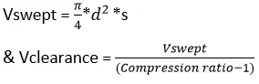
Where,
d = bore diameter in m
And s = stroke length in m
At the beginning, piston is at B.D.C hence volume at state 1 is taken as the addition of swept volume and clearance volume, simultaneously volume at state 2 is taken as clearance volume when piston reaches to B.D.C
Due to isentropic process 1-2, pressure and temperature at state 2 is calculated from the given input parameters by the formula,
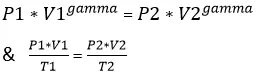
Process 2-3 is an isochoric process, hence Volume at state 2 and state 3 is constant.
Temperature at state 3 is also given from which pressure at state 3 is calculated by the formula,
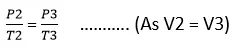
Process 3-4 is the isentropic expansion and volume at state 4 is equal to volume at state 1 because of isochoric process, pressure and temperature at state 4 is calculated by,
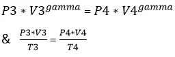
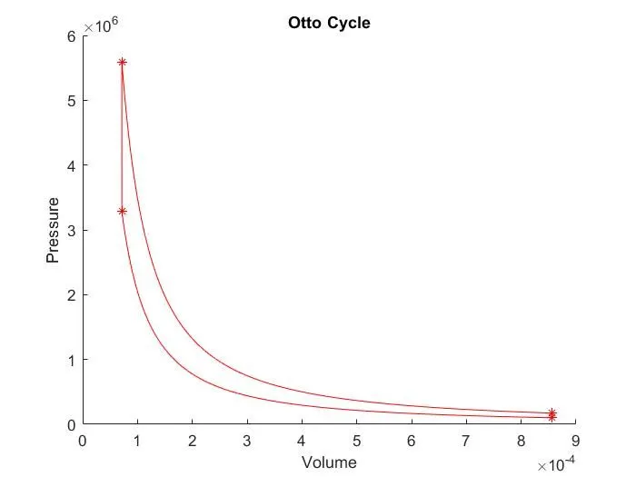
From this eqauations, points at state 1, 2, 3 & 4 are plotted. As Process 2-3 & Process 4-1 are constant volume processes, points of this processes in the Pressure- Volume diagram are joined by a straight line.
In order to determine the exact graph of compression and expansion, for each degree of rotation of crank, theta is varied and the instantaneous volume at each degree of crank angle is calculated by the formula,

Where,
R = Connecting rod ratio = Connecting rod length/Crank radii.
This formula is calculated in a function & that function is called in the main program. To simplify the code, this formula is broken into Term1, Term2 and Term3.
Function to calculate the instantaneous volume at each degree of rotation of crank,
function[V] = function_piston_kinematics_otto_cycle(bore,stroke,comp_ratio,Connecting_rod,Start_crank,End_crank)

Crank_radii = stroke/2;
Connect_rod_ratio = Connecting_rod/Crank_radii;

Vswe = (pi/4)*bore^2*stroke;
Vcle = Vswe/(comp_ratio-1);

theta = linspace(Start_crank,End_crank,720);

Term1 = 0.5*(comp_ratio-1);
Term2 = Connect_rod_ratio+1-cosd(theta);
Term3 = (Connect_rod_ratio^2 - sind(theta).^2).^0.5;

V = Vcle.*(1+ Term1*(Term2 - Term3));
end
From this function, instantaneous volume for expansion and compression is calculated by calling the function in main program only start angle and end angle of crank is given a differently for compression and expansion stroke according to position of piston. Then, constant from the other processes is calculated by the formula,

And with the same constant, instantaneous pressure at each degree of rotation of crank is calculated by the same formula for expansion and compression with taking instantaneous volume values at each degree of rotation of the crank, results of process 1-2 & 3-4 has been plotted by plotting this instantaneous pressure and volume values at each degree of rotation of crank.
Results –
Efficiency of Otto cycle is calculated by a formula,
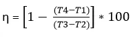
Efficiency of this Otto cycle problem is calculated as 62.9893%
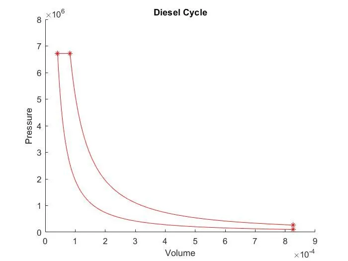
2. Diesel Cycle –
Diesel cycle is also called constant pressure cycle, in which heat addition process is isobaric process and heat rejection takes place at constant volume.
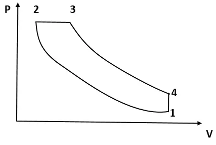
Where,
Process 1-2 – Isentropic compression
Process 2-3 – Isobaric Heat Addition
Process 3-4 – Isentropic Expansion
Process 4-1 – Isochoric Heat Rejection
Code to generate Pressure-Volume diagram of Diesel cycle –
%Diesel cycle

%Inputs
gamma= 1.4;

%State Variables
P1 = 101325
T1 = 500


%Engine Geometry Parameters
bore = 0.1;
stroke = 0.1;
Connecting_rod = 0.15;
comp_ratio = 20;
cutoff_ratio = 2;
%Calculations of Swept Volume and Clearance Volume
Vswe = (pi/4)*bore^2*stroke
Vcle = Vswe/(comp_ratio-1)

%State variables at pt1
V1 = Vswe + Vcle
V2 = Vcle

%State variables at pt 2
%Calculate P2 by P1V1^gamma = P2V2^gamma; P2 = P1V1^gamma/V2^gamma
P2 = P1*(V1/V2)^gamma

%Calculate T2 by PV/T = const; P1V1/T1 = P2V2/T2
T2 = P2*V2*T1/(P1*V1)

%Callimg the Function for compression
V_compression = function_piston_kinematics_otto_cycle(bore,stroke,comp_ratio,Connecting_rod,180,360);
constant_c = P1*V1^gamma;
P_compression = constant_c./V_compression.^gamma;

%state variables at pt 3;
P3 = P2

%Calculate V3 by cut-off ratio.
V3 = cutoff_ratio*V2
%calculate T3 by PV/T = const; P2V2/T2 = P3V3/T3
T3 = (V3*T2)/V2

%State variables at pt. 4;
V4 = V1

%Calculate P4 by P3V3^gamma = P4V4^gamma
P4 = P3*(V3/V4)^gamma

%calculate T4 by P3V3/T3 = P4V4/T4
T4 = P4*V4*T3/(P3*V3)

%Calling the Function for Expansion
V_expansion = function_piston_kinematics_otto_cycle(bore,stroke,comp_ratio,Connecting_rod,383,540);
constant_c = P3*V3^gamma;
P_expansion = constant_c./V_expansion.^gamma;

% Efficiency calculation
Eff = [(1-(1/comp_ratio^(gamma-1))*(cutoff_ratio^gamma/(gamma*(cutoff_ratio-1))))]*100
%Plotting
hold on
plot(V1,P1, '*','color','r')
plot(V2,P2, '*','color','r')
plot(V_compression,P_compression,'color','r')
plot(V3,P3, '*','color','r')
plot(V_expansion,P_expansion,'color','r')
plot(V4,P4, '*','color','r')
plot([V2 V3],[P2 P3],[V4 V1],[P4 P1], 'Linewidth',0.5,'color','r')
axis([0 9*10^-4 0 8*10^6])
xlabel('Volume');
ylabel('Pressure');
title('Diesel Cycle')
Explanation –
Along with the compression ratio, cut-off ratio is taken as an input in Diesel cycle, which is the ratio of Volume after heat addition to the volume before heat addition.
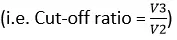
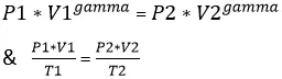
Here only pressure and temperature at state 1 is given as an input. Cut-off ratio is assumed as 2 and compression ratio for diesel engine is assumed as 20. Due to isentropic process 1-2, pressure and temperature at state 2 is calculated from the given input parameters by the formula,
Process 2-3 is an isobaric process, hence pressure at state 2 and state 3 is constant.
Volume at point 3 is calculated by the formula,
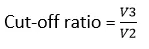
Temperature at state 3 is calculated by the formula,

Process 3-4 is the isentropic expansion and volume at state 4 is equal to volume at state 1 because of isochoric process, pressure and temperature at state 4 is calculated by,
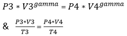
From this equations, points at state 1, 2, 3 & 4 are plotted. As Process 2-3 is isobaric process & Process 4-1 is constant volume processes, points of this processes in the Pressure- Volume diagram are joined by a straight line.
In order to determine the exact graph of compression and expansion, for each degree of rotation of crank, theta is varied and the instantaneous volume at each degree of crank angle is calculated by the same formula as of Otto cycle,

Where,
R = Connecting rod ratio = Connecting rod length/Crank radii.
This formula is calculated in a function & that function is called in the main program. To simplify the code, this formula is broken into Term1, Term2 and Term3.
The formula and function for otto cycle and diesel cycle remains same as it depends on the degree of rotation of crank, compression ratio, crank radii and clearance volume.
Due to injection delay (late fuel injection in diesel engine), start crank angle for expansion stroke is taken 23 degrees later. (i.e. 383 degrees). Injection delay is assumed as 23 degrees.
From the same function as of otto cycle, instantaneous volume for expansion and compression is calculated by calling the function in main program only start angle and end angle of crank is given a differently for compression and expansion stroke according to position of piston. Then, constant from the other processes is calculated by the formula,

And with the same constant, instantaneous pressure at each degree of rotation of crank is calculated by the same formula for expansion and compression with taking instantaneous volume values at each degree of rotation of the crank, results of process 1-2 & 3-4 has been plotted by plotting this instantaneous pressure and volume values at each degree of rotation of crank.
Results –
Efficiency of diesel cycle is given as,

Efficiency of this Diesel cycle problem is calculated as 43.1275%