Simulation of a simple pendulum using ordinary differential equation in MATLAB.

Aim – To solve the ordinary equation of simple pendulum using ODE 45 command and to generate the simulation of simple pendulum by using MATLAB code.

Introduction – Ordinary differential equations are used to describe the motion of a system. A system could be mechanical, electrical, thermal etc. Solving the differential equation can give the description of a system motion. In order to solve the ordinary differential equations of a higher order, first differential equation should be broken into first order equation by assuming some variables, to solve the equation easily.

Ordinary differential equation for simple pendulum is,

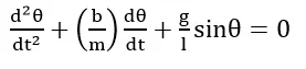
Where,

b = damping coefficient

m = mass of pendulum in Kg

g = gravity of acceleration in m/sec^2

theta (θ) = angular velocity in m/sec.

In order to simplify the differential equation, this ordinary differential equation is converted into first order equation by assuming,

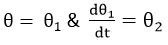
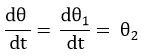
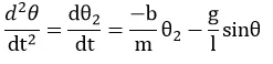
By using this equations, MATLAB code has been written.

Code for Simulation of Simple Pendulum using ODE45

%ODE 45 Simple Pendulum
clear all
close all
clc

%Input Parameters
m = 0.1;
b = 0.05;
L = 1;
g = 9.81;

theta_input = [0;3];

%Time
t_span = linspace(0,20,500);

%ODE 45
[t,results] = ode45(@(t,theta) ode45_function(t,theta,m,b,L,g), t_span, theta_input);

%Plot
figure(1);
plot(t,results);
xlabel('Time');
ylabel('Displacement');
title('ODE 45 Simple Pendulum')
legend('Diplacement','Velocity')
grid on

ct =1;
for i = 1:length(results)
    Results = results(i);
    x0 = 0;
    y0 = 0;
    
    x1 = sin(Results);
    y1 = -cos(Results);

    
    figure(2)
    plot([x0 x1],[y0 y1],'linewidth',2,'color','g');
    hold on
    plot(x1,y1,'o','markerfacecolor','r')
    hold off
    
    xlabel('Time')
    ylabel('Displacement')
    grid on
    axis([-0.8 0.8 -1.2 0])
    K(ct) = getframe(gcf)
    ct = ct+1
    pause(0.001)
end
   
movie(K)
videofile = VideoWriter('simple_pendulum_ode.avi','uncompressed AVI');
open(videofile)
writeVideo(videofile,K)
close(videofile)
    

Explanation –

After getting the first order differential equation with certain assumptions, input parameters are taken as mass = 1 kg, damping coefficient = 0.5 & length of pendulum = 1m. Initial angular displacement is taken as 0 rad/sec and initial angular velocity is taken as 3 rad/sec. The motion of a simple pendulum is simulated for 0 to 20 sec with 500 parts between the given time.

Ordinary differential equation is solved in the MATLAB by the command ODE45. The function, in which ordinary differential equation is broken into first order differential equation and is called in the main program. To implement the ODE45 command, outputs are given as results with respect to time (i.e. Displacement and Velocity) and is equate to the ODE 45 command as a function of t and theta with calling the function in main program at given angular displacement, angular velocity at given time.

Function to call in the main program –

function[dtheta_dt] = ode45_function(t,theta,m,b,L,g)

theta1 = theta(1)
theta2 = theta(2)

dtheta1_dt = theta2;
dtheta2_dt = (-b/m)*theta2 - (g/L)*sin(theta1);
dtheta_dt = [dtheta1_dt; dtheta2_dt];
end

From the function, various converted first order values of displacement and velocity are obtained and ODE45 function is implemented. Results are plotted in the 2 figures.

In first figure, angular displacement and angular velocity is plotted vs time. Legend command is used to differential the angular displacement and angular velocity with respect to time.

To simulate the motion of a simple pendulum, initially counter is taken as 1 is incremented at the end of each loop and then pause command is implemented. With the markerface command, end of the pendulum is given in red color.

In for loop, the results of angular velocity and angular displacement are plotted serially with increment of 1 after each loop, so that individual frames of each figure is obtained. Link endpoints are calculated with trigonometric relations.

Results –

Figure 1 – Angular Displacement and Angular Velocity vs Time

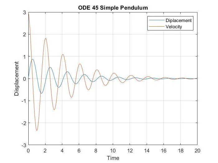
Figure 2 – Animation of a simple pendulum using ODE45