Week 4.1 - Genetic Algorithm

%concept of genetic algorithm and understanding the stalagmite function.

%INPUTS ARRAYS
X=linspace(0,0.6,150);
y=linspace(0,0.6,150);

[X,Y]=meshgrid(x,y);    %returns 2-D grid coordinates based on the coordinates contained in vectors x and y

 % evaluating stalagmite function
 for i=1:length(X)
     for j=1:length(Y)
         inp(1)=X(i,j)
         inp(2)=Y(i,j)
         f(i,j)=stalagmite_func(inp)
     end
 end

 %PLOTING 3D SURFACE
 figure(1)
 surfc(X,Y,f)
 shading interp
 xlabel('x value')
 ylabel('y value')
 [inputs,fval]=ga(@stalagmite_func,2);%GA Inbuilts command giving the optimiztion
                                       %value of the fuction as by giving x and y inputs
                                       
                                       

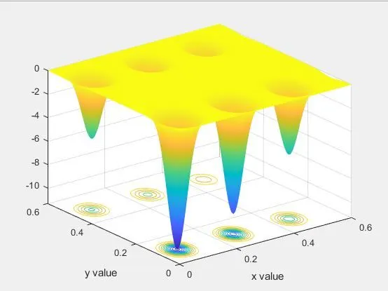
%Each time we are excuting GA gives different value so to know exact optmization value we study 3 different cases          

%STUDY1 STATICAL BEHAVIOUR
num_cases=50;
tic
 for i=1:num_cases
     [inputs,fopt(i)]=ga(@stalagmite_func,2);%GA give the  INPUTS where we can get optimisation value 
     xopt(i)=inputs(1);
     yopt(i)=inputs(2);
 end
 Time_Study=toc
 figure(2)
 subplot(2,1,1)
 hold on
 surfc(x,y,f)
 shading interp
 plot3(xopt,yopt,fopt,'marker','o','markersize',5,'markerfacecolor','r')
 title('unbounded inputs')
 subplot(2,1,2)
 plot(fopt)
 xlabel('iterations')
 ylabel('function minimum')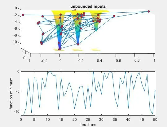

%STUDY2 STATICAL BEHAVIOUR WITH UPPER AND LOWER BOUND
 num_cases=50;
 tic
 for i=1:num_cases;
    [inputs,fopt(i)]=ga(@stalagmite_func,2,[],[],[],[],[0;0],[1;1]);
    xopt(i)=inputs(1);
    yopt(i)=inputs(2);
 end
 study_time2=toc
 figure(3)
 subplot(2,1,1)
 hold on
 surfc(x,y,f)
 shading interp
 plot3(xopt,yopt,fopt,'marker','o','markersize',5,'markerfacecolor','r')
 title('bounded inputs')
 subplot(2,1,2)
 plot(fopt)
 xlabel('iteration')
 ylabel('function minimum')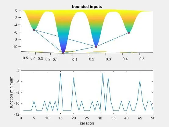

% STUDY 3 INCREASING GA ITERATION
 options=optimoptions('ga');
 options=optimoptions(options,'populationsize',250)
 tic
 num_cases=50;
 for i=1:num_cases;
    [inputs,fopt(i)]=ga(@stalagmite_func,2,[],[],[],[],[0;0],[.4;.4],[],[],options);
    xopt(i)=inputs(1)
    yopt(i)=inputs(2)
 end
 study_time3=toc
 figure(4)
 subplot(2,1,1)
 hold on
 surfc(x,y,f)
 shading interp
 plot3(xopt,yopt,fopt,'marker','o','markersize',5,'markerfacecolor','r')
 title('bounded inputs')
 subplot(2,1,2)
 plot(fopt)
 xlabel('iteration')
 ylabel('function minimum')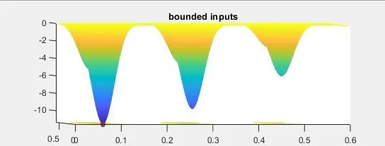

genetic algorithm

A genetic algorithm (GA) is a method for solving both constrained and unconstrained optimization problems based on a natural selection process that mimics biological evolution.

The algorithm repeatedly modifies a population of individual solutions.

It is an area of study, that deals with , how to minimize or maximize a particular function , which depends on multiple parameters.

GA is an optimization process and optimization is a decision making process, helps to find best results. It maximise the factors productivity, strength, reliability, efficiency, utilization.

GA SYNTAX

x = ga(fun,nvars)

x = ga(fun,nvars,A,b)

x = ga(fun,nvars,A,b,Aeq,beq)

x = ga(fun,nvars,A,b,Aeq,beq,lb,ub)

x = ga(fun,nvars,A,b,Aeq,beq,lb,ub,nonlcon)

x = ga(fun,nvars,A,b,Aeq,beq,lb,ub,nonlcon,options)

x = ga(fun,nvars,A,b,[],[],lb,ub,nonlcon,IntCon)

x = ga(fun,nvars,A,b,[],[],lb,ub,nonlcon,IntCon,options)

x = ga(problem)

[x,fval] = ga(___)

[x,fval,exitflag,output] = ga(___)

[x,fval,exitflag,output,population,scores] = ga(___)

Description

1-: x = ga(fun,nvars) finds a local unconstrained minimum, x, to the objective function, fun. nvars is the dimension (number of design variables) of fun.

Note

Passing Extra Parameters explains how to pass extra parameters to the objective function and nonlinear constraint functions, if necessary.

example

2-: x = ga(fun,nvars,A,b) finds a local minimum x to fun, subject to the linear inequalities A*x ≤ b. ga evaluates the matrix product A*x as if x is transposed (A*x').

example

3-: x = ga(fun,nvars,A,b,Aeq,beq) finds a local minimum x to fun, subject to the linear equalities Aeq*x = beq and A*x ≤ b. (Set A=[] and b=[] if no linear inequalities exist.) ga evaluates the matrix product Aeq*x as if x is transposed (Aeq*x').

example

4-: x = ga(fun,nvars,A,b,Aeq,beq,lb,ub) defines a set of lower and upper bounds on the design variables, x, so that a solution is found in the range lb ≤ x ≤ ub. (Set Aeq=[] and beq=[] if no linear equalities exist.)

example

5-: x = ga(fun,nvars,A,b,Aeq,beq,lb,ub,nonlcon) subjects the minimization to the constraints defined in nonlcon. The function nonlcon accepts x and returns vectors C and Ceq, representing the nonlinear inequalities and equalities respectively. ga minimizes the fun such that C(x) ≤ 0 and Ceq(x) = 0. (Set lb=[] and ub=[] if no bounds exist.)

example

6-: x = ga(fun,nvars,A,b,Aeq,beq,lb,ub,nonlcon,options) minimizes with the default optimization parameters replaced by values in options. (Set nonlcon=[] if no nonlinear constraints exist.) Create options using optimoptions.

example

7-: x = ga(fun,nvars,A,b,[],[],lb,ub,nonlcon,IntCon) or x = ga(fun,nvars,A,b,[],[],lb,ub,nonlcon,IntCon,options) requires that the variables listed in IntCon take integer values.

Note

When there are integer constraints, ga does not accept linear or nonlinear equality constraints, only inequality constraints.

8-: x = ga(problem) finds the minimum for problem, a structure described in problem.

9-: [x,fval] = ga(___), for any previous input arguments, also returns fval, the value of the fitness function at x.

10-: [x,fval,exitflag,output] = ga(___) also returns exitflag, an integer identifying the reason the algorithm terminated, and output, a structure that contains output from each generation and other information about the performance of the algorithm.

11-: [x,fval,exitflag,output,population,scores] = ga(___) also returns a matrix population, whose rows are the final population, and a vector scores, the scores of the final population.