Week 4.1 - Genetic Algorithm
1. AIM
The aim of this challenge is to write a code for optimising stalagmite function using genetic algorithm and then explain the genetic alogorithm
2. Theory
Optimisation is a process used to find out the best suitable values for the variables which satisfies the constraints and also are well within the variable boundaries. We want to get the most suitable solution for a problem which is satisfying the inputs conditions given to us. Examples will be increasing the profit under a given set of conditions or reducing the time taken for a process.
Different algorithms are used to optimise the function and one of which is the genetic algorithm which takes refernce from darwin's theory of evolution.
Genetic algorithm is a search based optimisation techniques and is inspired by darwin's theory of evolution. In this the fittest offsprings are selected for producing the next generation.
Process of natural Selection
In this first the fittest individuals are selected from a population and they produce offsprings which are more fit than the parents. This process keeps on iterating until the fittest individuals are found.
The same principle is implemented to a mathematical problem in which a set of solutions for a problem is optimised to get the best one.
There are five phases in this are
Initial population
Fitness function
Selection
Crossover
Mutation
Initial Population
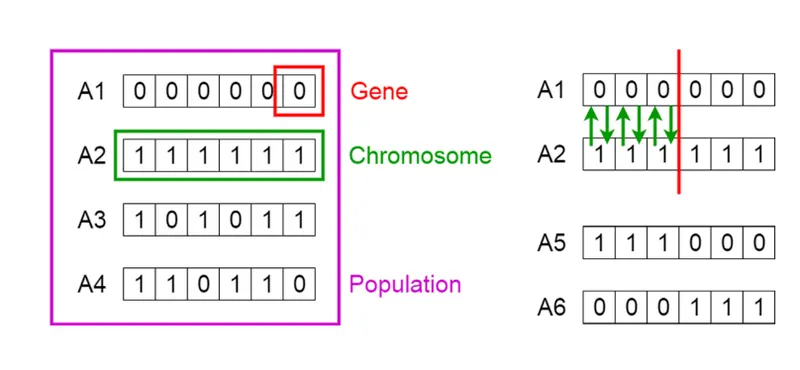
The process starts with a set of individuals called population Each individual is the solution to the problem
Every individual will have a set of characterestics called Genes(variables) which are joined in to a string to form a chromosome(solution)
Fitness function
This defines the fitness level of individuals. the probability of their selection is based on this fitness score.
Selection
The idea of the selection phase is to select the fittest individuals and let them pass their genes to the next generation. The main goal of this phase is to find the region where the chances of getting the best solution are more.
Crossover
Crossover is a way of reproduction. A random point is selected when a pair of parents reproduce. offsprings are created by exchanging the genes of parents up to the crossover point.
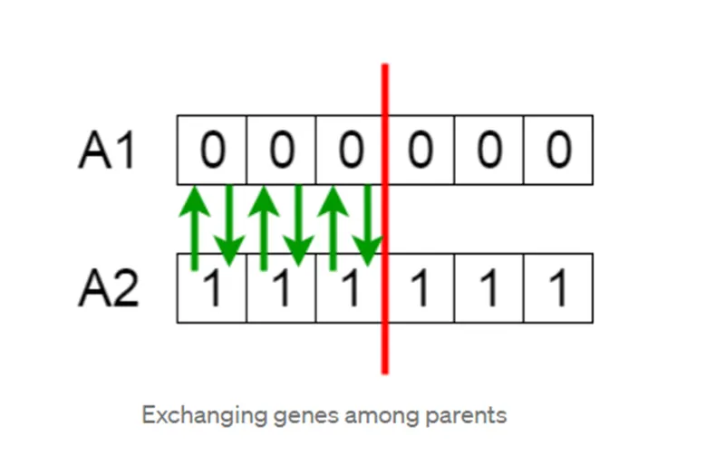
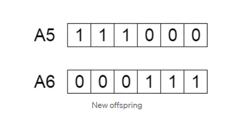
Three types of crossover are there.
Single point crossover
Two-point crossover
Uniform crossover
Mutation
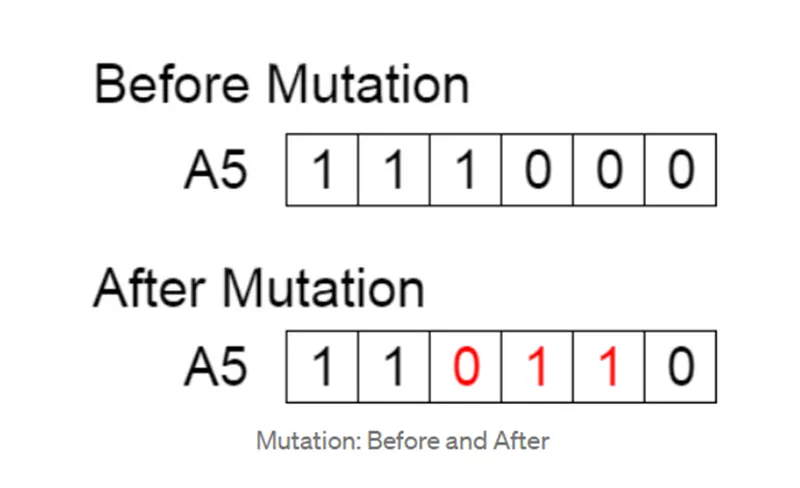
In certain offsprings, some of their genes undergo mutation and the gene strings get flipped. Mutation is important since it will ensure to maintain the diversity within the population.
The Syntax of genetic algorithm is
[x,fval]= ga(fun,nvars,A,b,Aeq,beq,lb,ub,nonlcon,intcon,options)
Where
‘x’ is the local unconstrained minima
‘fval’ returns with the value of fitness function at x
‘fun’ is the objective function
‘nvars’ is the dimension of fun (number of design variables)
‘A’&’b’ are the linear inequalities `A*x<=b`
'Aeq' & 'beq' are the linear equalities `Aeq*x=beq`
'lb' & 'ub' lower and upper bounds of design variables
'nonlcon' non linear function which returns with the non linear equality and inequality
'intcon' the variable takens a integer value
'optioins' can specify the optimization options like population size
Stalagmite Function
A stalagmite is a type of rock formation which rises from the floor of a cave due to deposited material accumulation 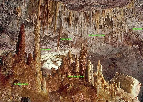
The stalagmite function is defined as
`f(x,y)=f_1(x)*f_2(x)*f_1(y)*f_2(y)`
`f_1(x)=[sin(5.1*pi*x+0.5)]^6`
`f_1(y)=[sin(5.1*pi*y+0.5)]^6`
`f_2(x)=exp[-4*ln(2)*((x-0.667)^2/0.64)]`
`f_2(y)=exp[-4*ln(2)*((y-0.667)^2/0.64)]`
3. Code Explanation
First we write the stalagmate function as per the equations given above
%stalagmite function
function f=ga_stalagmite(input);
x=input(1);
y=input(2);

f1x=[sin(5.1*(pi).*x+0.5)].^6;
f1y=[sin(5.1*(pi).*y+0.5)].^6;
f2x=exp(((-4)*log(2).*(x-0.0667).^2)./0.64);
f2y=exp(((-4)*log(2).*(y-0.0667).^2)./0.64);
f=-(f1x*f1y*f2x*f2y);
end
genetic algorithm is used to find out the minimum value of the function. So in order to find out the maximum value of the function, we need to modify the stalagmite function by multiplying it with -1.
Now if we execute the ga algorithm to optimise the stalagmite function and run the code we will get different values each time
clear all
close all
clc

%Inputs
x=linspace(0,0.6,150);
y=linspace(0,0.6,150);

%Creating 2D mesh
[xx,yy]=meshgrid(x,y);


%Evaluating function
for i=1:length(xx)
    for j=1:length(yy)
        input(1)=xx(i,j);
        input(2)=yy(i,j);
        f(i,j)=ga_stalagmite(input);
    end
end

%Applying ga algorithm
    [input, fval]=ga(@ga_stalagmite,2);

%Plotting results
surfc(xx,yy,f);
shading interp;
xlabel('x-axis');
ylabel('y-axis');
disp(input)
disp(fval)
here only inputs are given for the function and it is not the boundary for optimisation.
2D mesh created by meshgrid
Now we evaluate the function for the entire value of x & y using for loop
Now the function is optimised by ga and we define only the number of variables.
surface plot used to plot the values of x,y & f.
the values for inputs and function are displayed.
3.1 optimising the function in a unbounded region (also runnign the algorithm multiple times to understand the results)
The algorithm is ran for 50 times and the function maxima is plotted against the iterations.
Initial potion of the code is same. The total number of cases is defined as 50. for loop used to execute the algorithm 50 times. the optimum values for x&y are obtained frominput and the otimum value for the function is also calculated
tic-toc command used to count the time taken to execute the function. tic command stores the time at that moment and toc command calculates the duration from the stored value.
the subplot command is used to plot multiple plots in single figure window. here we are plotting the 3D surface plot and also the function maxima vs iteration .
In the first figure, we plot the surface plot as explained earlier. Now we plot the 3D points of the optimum values of x,y and function value. This will mark all the optimum values on the surface. the title and axis labels for this plot is given and then we plot the second plot.
This plot is function maxima vs iterations. so we plot fopt. And the axis labels are mentioned.
3.2 Definfing upper and lower bounds for the optimisation function
In this we define the optimisation function to run within a boundary. Lower bound for x&y is taken as 0 and upper bound as 1.
in ga syntax, if we are not defining any inbetween parameters, then we can simply give a empty square bracket to represent it.
The time calculated is displayed for all 3 studies
3.3 Increasing the population size
Optimumoptions command used to specify the population size of ga.
The Final code for all the studies are as follows
clear all
close all
clc

%Inputs
x=linspace(0,0.6,150);
y=linspace(0,0.6,150);
%Number of times the function is to be calculated(iterations)
num_cases=50;

%Creating 2D mesh
[xx,yy]=meshgrid(x,y);


%Evaluating function
for i=1:length(xx)
    for j=1:length(yy)
        input(1)=xx(i,j);
        input(2)=yy(i,j);
        f(i,j)=ga_stalagmite(input);
    end
end

%Study 1 Optimising the function without any specified boundary
tic
for i=1:num_cases
    [input, fopt(i)]=ga(@ga_stalagmite,2);
    xopt(i)=input(1);
    yopt(i)=input(2);
end
Time_1=toc;
figure(1)
%creating multiple plots in one figure
%defining first plot
subplot(2,1,1);
hold on;
surfc(xx,yy,f);
shading interp;
%for plotting a 3D point
plot3(xopt,yopt,fopt,'marker','o','MarkerSize',5,'MarkerFaceColor','r');
title('Unbounded inputs');
xlabel('x-axis');
ylabel('y-axis');
%defining second plot
subplot(2,1,2)
plot(fopt);
xlabel('Iterations');
ylabel('function maxima');


%Study 2 Optimising the function with specified boundary
tic
for i=1:num_cases
    [input, fopt(i)]=ga(@ga_stalagmite,2,[],[],[],[],[0;0],[1;1]);
    xopt(i)=input(1);
    yopt(i)=input(2);
end
Time_2=toc;
figure(2)

%creating multiple plots in one figure
%defining first plot
subplot(2,1,1);
hold on;
surfc(xx,yy,f);
shading interp;
%for plotting a 3D point
plot3(xopt,yopt,fopt,'marker','o','MarkerSize',5,'MarkerFaceColor','r');
title('Unbounded inputs');
xlabel('x-axis');
ylabel('y-axis');
%defining second plot
subplot(2,1,2)
plot(fopt);
xlabel('Iterations');
ylabel('function maxima');

%Study 3 Increasing the population size

options=optimoptions('ga');
options=optimoptions(options,'PopulationSize',200);

tic
for i=1:num_cases
    [input, fopt(i)]=ga(@ga_stalagmite,2,[],[],[],[],[0;0],[1;1],[],[],options);
    xopt(i)=input(1);
    yopt(i)=input(2);
end
Time_3=toc;

figure(3)
%creating multiple plots in one figure
%defining first plot
subplot(2,1,1);
hold on;
surfc(xx,yy,f);
shading interp;
%for plotting a 3D point
plot3(xopt,yopt,fopt,'marker','o','MarkerSize',5,'MarkerFaceColor','r');
title('Bounded inputs with increased population size');
xlabel('x-axis');
ylabel('y-axis');
%defining second plot
subplot(2,1,2)
plot(fopt);
xlabel('Iterations');
ylabel('function maxima');

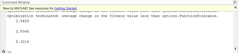
disp(Time_1)
disp(Time_2)
disp(Time_3)
4. Error observed
The error observed during coding
1. Only figure for 3rd study got displayed.
The number of figures were not specified in the code which resulted in displaying only the last figure. Rectified by specifying figure numbers.
2. Stalagmate function not modified.
ga is used to find the minima of a function. Stalagmate function not modified before optimising with ga giving a single fopt value of 0.
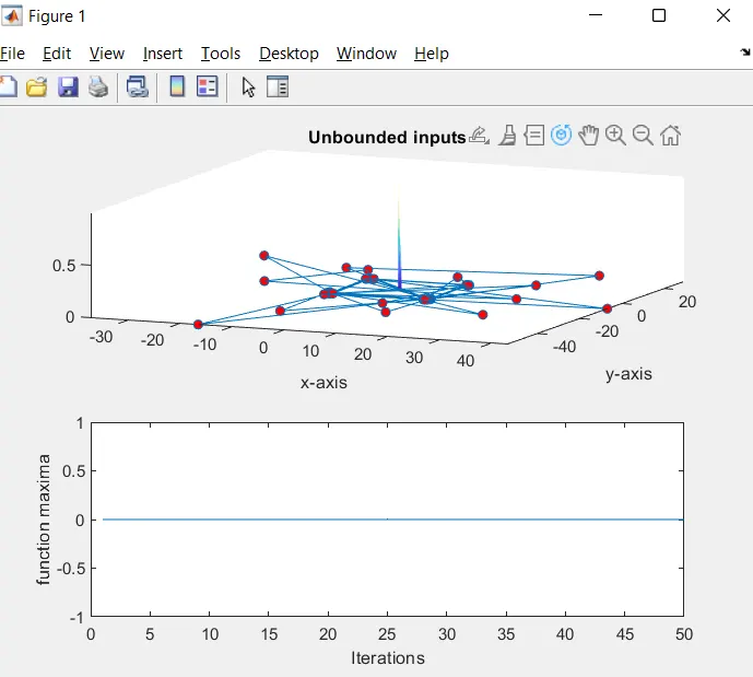
Issue resolved by adding a negative sign to stalagmate function
5. Final output
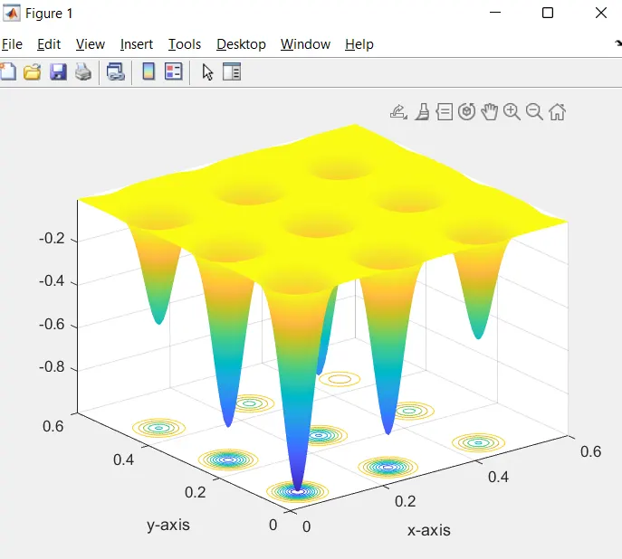
1. running the optimisation only once and finding fval
2. Optimising in unbounded condition (running 50 times)
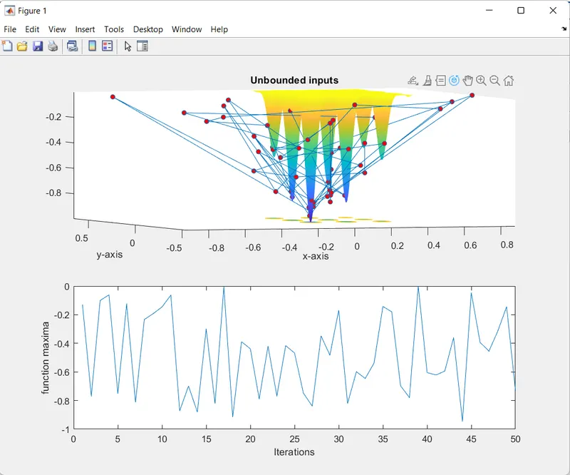
It can be found that the function is not taking inputs from within a boundary. Optimisation is not good at all since values are spreaded everywhere and any of these values can be the maxima
3. Running with a specified boundary
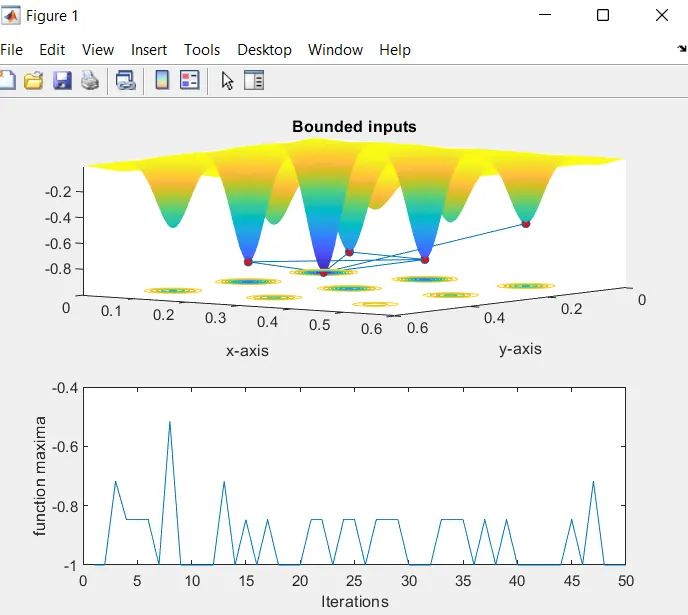
this is better than the previous study and inputs are taken well within the boundary
4. Optimising by increasing the population size
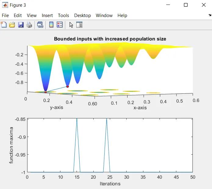
Only two optimum points where the function is maximum.
The time taken for running all 3 studies is displayed in order
6. References
https://www.tutorialspoint.com/genetic_algorithms/genetic_algorithms_introduction.htm