Week 3 - Solving second order ODEs

1. Aim

To write a program to solve the differential equation for the motion of a simple pendulum and create a animation for the simple pendulum movement

2.Theory

Differential equations explains the relation between two or more functions and their derivatives. In real life applications can be used to define the relation ship between physical quantities and their rate of changes. For a simple pendulum, the differential equation defines the relation ship between the angle and time. The differntial equation for the simple pendulm is given as

`(d^2theta)/dt^2+b/m*(d theta)/dt+g/lsintheta=0`

Given

b=damping coefficient

m=mass of ball in kg

g=gravity in m/s^2

l=length in m

For solving this differential equation in 2nd order, it needs to be broken down in to 2 differential equation with order 1.

Lets consider `theta=theta_1` then

`(d theta)/dt=(d theta_1)/dt=theta_2`

`(d^2theta)/dt=(d^2theta_1)/dt=d/dt (d theta_1)/dt=(d theta_2)/dt`

So the main equation becomes,

`(d theta_2)/dt+b/m*theta_2+g/l*sintheta_1=0`

`(d theta_2)/dt=-b/m*theta_2-g/l*sintheta_1`

So the original diffrential equation of 2nd order is convetred into two differential equations of order 1

`d/dt[[theta_1],[theta_2]]=[[theta_2],[-b/mtheta_2-g/lsintheta_1]]`

Since these are differential equations in order 1, these can be solved by the ODE45 function in MATLAB.

3. Code Explanation

First, we need to create the code for the function which will represent the 2 differential equations

The function dtheta_dt has t and theta as the major inputs along with m,b,l,and g.

Since the solution will be a 2 column matrix, we need to define theta_1 and theta_2

theta_1 will be the first solution of theta (theta(1))

theta_2 will be the second solution of theta (theta(2))

Now we define the relations for dtheta_1/dt and dtheta_2/dt as mentioned above in theory section

Once bothe relations are defined, we define dtheta/dt which is the column matrix of dtheta_1/dt and dtheta_2/dt

%differential equation function
function[dtheta_dt]=function_ODE(t,theta,b,l,g,m)

theta1=theta(1);
theta2=theta(2);
dtheta1_dt=theta2;
dtheta2_dt=(-b/m)*theta2-(g/l)*sin(theta1);
dtheta_dt=[dtheta1_dt; dtheta2_dt];
end

Now we create the program to solve the differntial equation and plot the results and also create the animation for the

pendulum motion

As always we start with clear all, close all and clc

We define the inputs as mentioned in the question

Now, we define the initial conditions for the problem. here we define both displacement and velocity of the mass. As per question, displacement is 0 and velocity is 3rad/s

Now, the time span is defined and number of instances were we need to calculate the solutions. The total time span is 20 s and we are dividing it equally in to 500 instances with linspace command

the ode function is given in the next step. The equation is depends on theta and time. so they are defined first and then the function created earlier is called here inside the ode45 syntax. Also the time span is given as the limits of integration and the initial conditions as refernce point from where the calculation needs to start.

Now we plot the results. in the first figure, the solution in the first instance of the matrix is plotted against time.

hold on command is used to plot the second solution also against time in the same plot.

labels, title and legends are provided for the plot created.

Now for creating the second figure, let give a counter for the frame as F.

for loop is created to create iterations equal to the number of solutions.

Initial point for the thread is taken as (0,0). The final points will be the sin and cos components of l for the specified angle. For each value of theta the x1 & y1 points are calculated.

A horizontal line is drawn for the upper reference line. hold is switched on to plot multiple lines.

Line is drawn from initial poin to x1,y1. linewidth and color is specified.

axis limits are given and a marker is drawn at x1,y1 for indicating the mass.

pause used to slow down the code execution

An array M is created to record each frame. hold off applied to remove the initially created plot for the next point.

Increment is given to the frame F variable.

Now an array is created with all the frames ploted which will be equal to the number of solutions

movie is created to create the animation. videowriter command used to create an avi file , then open the videofile, then write the video into the file and close

%Solving differential equations with ODE45 function
clear all
close all
clc

%Inputs
l=1;
m=1;
b=0.05;
g=9.81;

%Initial condition
theta_0=[0;3];
%Time span
t_span=linspace(0,20,500);

%Differential equation solver
[t,solution]=ode45(@(t,theta) function_ODE(t,theta,b,l,g,m),t_span,theta_0);

%Plotting the results
figure(1);
plot(t,solution(:,1))
hold on
plot(t,solution(:,2))
ylabel('plot');
xlabel('time')

%Plotting the position of pendulum at every instatnt
F=1;
figure(2);

for i=1:length(solution)
    
    x_0=0;
    y_0=0;
    x_1=l*sin(solution(i,1));
    y_1=-l*cos(solution(i,1));
    plot([-2,2],[0,0]);
    hold on
    plot([x_0 x_1],[y_0 y_1],'LineWidth',2,'Color','g');
   axis([-2 2 -2 2]);
    plot(x_1,y_1,'Marker','o','MarkerSize',15,'Color','r','MarkerFaceColor','r');
    pause(0.0001);
    M(F)=getframe(gcf);
    hold off
    F=F+1;
end

%creating the animation
movie(M)
videofile=VideoWriter('Pendulum.avi','Uncompressed AVI');
open(videofile);
writeVideo(videofile,M);
close(videofile);

%end of code

4. Error observed

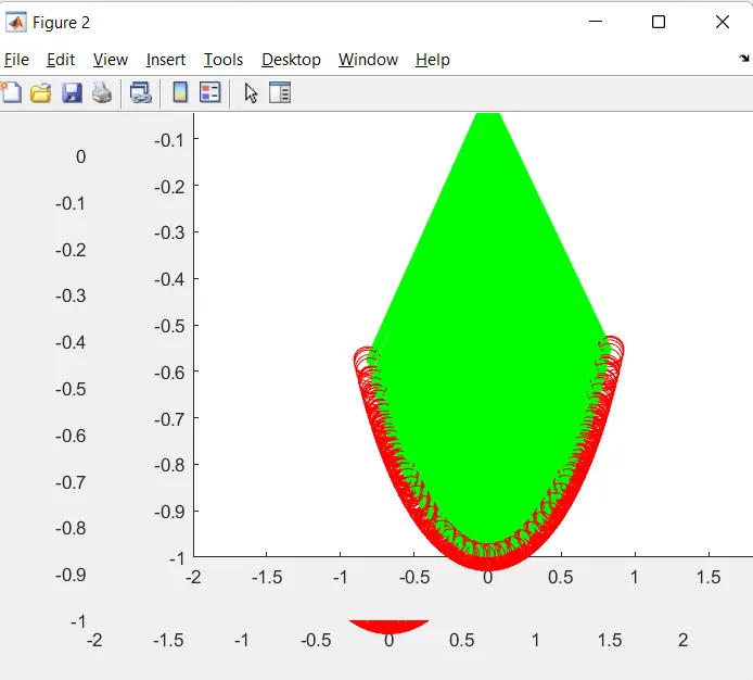
In this all the positions of pendulum is getting plotted since we added hold on command in the beginning and didn't switched it off . This was resolved by inserting hold off command

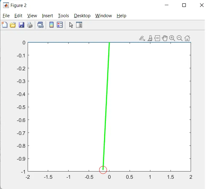
in this the axis values are not set. So the upper horizontal line is not visible. Also the marker is not filled. This is solved by specifying the axis values for both x and y axis.

5. Final result

The final result is a plot created in which both angular displacement and angular velocity is plotted as below.

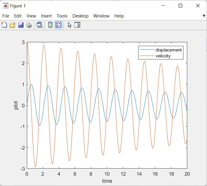
the second result is the animation created for the motion of a simple pendulum. the link for the video is as follows.

https://youtu.be/5irylVURiPw

6. Learning outcome

There are inbuilt functions in MATLAB which can be used to solve problems. ODE45 is a tool available in matlab for solving differential equations of 1st order.