Taylor Table Method and Matlab Code
# Objective
The objective of this project is to derive the central difference, skewed right-sided and skewed left-sided difference approximation for the second derivative using the Taylor table method.
compare the approximation errors and plot them for the above three different fourth-order approximation methods for the second derivative of function exp(x)*cosx using MATLAB.
#Central difference approximation
To get the fourth-order central difference approximation for the second derivative it is required to select five nodes.the second derivative approximate function,
`(del^2f)/(del^2x)=af(i-2)+bf(i-1)+cf(i)+df(i+1)+ef(i+2)`
To get these coefficients a,b,c,d,e it is required to expand each and every term using taylor series and convert them into five different linear equations.this can be done using the Taylor table,
Taylor Table:
| stencil | `f(i)` | `f'(i)*dx` | `f''(i)*dx^2` | `f'''(i)*dx^3` | `f''''(i)*dx^4` | `f'''''(i)*dx^5` | `f''''''(i)*dx^6` |
| a*f(i-2) | a | -2a | 2a | -4a/3 | 2a/3 | -32a/120 | 64a/720 |
| b*f(i-1) | b | -b | b/2 | -b/6 | b/24 | -b/120 | b/720 |
| c*f(i) | c | 0 | 0 | 0 | 0 | 0 | 0 |
| d*f(i+1) | d | d | d/2 | d/6 | d/24 | d/120 | d/720 |
| e*f(i+2) | e | 2e | 2e | 4e/3 | 2e/3 | 32e/120 | 64e/720 |
| Total | 0 | 0 | 1 | 0 | 0 |
a+b+c+d+e=0 --------(1)
-2a-b+d+2e=0 --------(2)
`2a+b/2+d/2+2e=1/dx^2` ------(3)
`-(4a)/3-b/6+d/6+(4e)/3=0` -----(4)
`(2a)/3+b/24+d/24+(2e)/3=0` -----(5)
These five linear equations can be solved using MATLAB if it is converted into matrix form.
`[[1,1,1,1,1],[-2,-1,0,1,2],[2,1/2,0,1/2,2],[-4/3,-1/6,0,1/6,4/3],[2/3,1/24,0,1/24,2/3]][[a],[b],[c],[d],[e]]=[[0],[0],[1],[0],[0]]`
solution using MATLAB
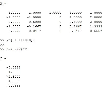
a=-0.0833
b=1.3333
c=-2.500
d=1.3333
e=-0.0833
Now second derivative using central difference approximation can be written as,
`(del^2f)/(del^2x)=(-f(x-2dx)+16f(x-dx)-30f(x)+16f(x+dx)-f(x+2dx))/(12*dx^2)`
- Now to proove that its fourth order approxiamtion,put the value of coefficients in the summation of taylor series expansion of different terms. First, third and fourth derivative term is zero because this is an approximation of second derivative.Now it turns out that fifth derivative terms also zero beacause of a=e and b=d.so, second derivative,sixth derivative and higher order to sixth derivative is remaining.
`(del^2f)/(del^2x)=(2a+b+d/2+2e)f''(x)*dx^2+((64a)/720+b/720+d/720+(64e)/720)f''''''(x)*dx^6+....`
deviding whole eqquation by dx^2 the maximum fourth order term is neglected.so its fourth order approximation.
Function in MATLAB
Now it is required to generate a function in MATLAB that can calculate the error between Numerical solution and Analytical solution of function exp(x)*cosx using above derived central difference fourth-order approximation formula.
% Fourth order central difference approximation of the second derivative
% Function=exp(x)*cosx

function central_diff_error=central_difference(x,dx)

% Analytical solution of function
Analytical_sol=-2*exp(x)*sin(x);

% Numerical solution using central difference approximation of the second derivative
Numerical_sol=(-(exp(x-2*dx)*cos(x-2*dx))+(16*exp(x-dx)*cos(x-dx))-(30*exp(x)*cos(x))+(16*exp(x+dx)*cos(x+dx))-(exp(x+2*dx)*cos(x+2*dx)))/(12*(dx)^2);

central_diff_error=abs(Analytical_sol-Numerical_sol);
end
# Skewed right sided difference approximation
For skewed sided difference approximation,
- Number of nodes=order of derivative+order of approximation
To get fourth order skewed right sided difference approximation for second derivative, six nodes needs to be selected.
`(del^2f)/(delx^2)=af(i)+bf(i+1)+cf(i+2)+df(i+3)+ef(i+4)+gf(i+5)`
Taylor table:
| stencil | f(i) | `f'(i)*dx` | `f''(i)*dx^2` | `f'''(i)*dx^3` | `f''''(i)*dx^4` | `f'''''(i)*dx^5` | `f''''''(i)*dx^6` |
| a*f(i) | a | 0 | 0 | 0 | 0 | 0 | 0 |
| b*f(i+1) | b | b | b/2 | b/6 | b/24 | b/120 | b/720 |
| c*f(i+2) | c | 2c | 2c | 4c/3 | 2c/3 | 4c/15 | 64c/720 |
| d*f(i+3) | d | 3d | 9d/2 | 27d/6 | 81d/24 | 243d/120 | 729d/720 |
| e*f(i+4) | e | 4e | 8e | 64e/6 | 256e/24 | 1024e/24 | 4096e/720 |
| g*f(i+5) | g | 5g | 25g/2 | 125g/6 | 625g/24 | 3125g/120 | 15625g/720 |
| Total | 0 | 0 | 1 | 0 | 0 | 0 |
This system of equations can be converted into matrix form to solve them using MATLAB.
`[[1,1,1,1,1,1],[0,1,2,3,4,5],[0,1/2,2,9/2,8,25/2],[0,1/6,4/3,27/6,64/6,125/6],[0,1/24,2/3,81/24,256/24,625/24],[0,1/120,4/15,243/120,1024/120,3125/120]][[a],[b],[c],[d],[e],[g]]=[[0],[0],[1],[0],[0],[0]]`
Solution:
a=3.750
b=-12.8333
c=17.8333
d=-13.0000
e=5.08333
g=-0.8333
Now second derivative using skewed right sided difference approximation can be written as,
`(del^2f)/(del^2x)=(45f(x)-154f(x+dx)+214f(x+2dx)-156f(x+3dx)+61f(x+4dx)-10f(x+5dx))/(12*dx^2)`
Function in MATLAB
Now it is required to generate a function in MATLAB that can calculate the error between Numerical solution and Analytical solution of function exp(x)*cosx using above derived skewed right-sided difference fourth-order approximation formula.
% Skewed right sided fourth order approximtion of second derivative
% Function=exp(x)*cosx

function Skewed_right_sided_error=skewed_right_sided_difference(x,dx)

% Analytical solution of function
Analytical_sol=-2*exp(x)*sin(x);

% Numerical solution using right-sided difference approximation of the second derivative
Numerical_sol=((45*exp(x)*cos(x))-(154*exp(x+dx)*cos(x+dx))+(214*exp(x+2*dx)*cos(x+2*dx))-(156*exp(x+3*dx)*cos(x+3*dx))+(61*exp(x+4*dx)*cos(x+4*dx))-(10*exp(x+5*dx)*cos(x+5*dx)))/(12*(dx)^2);

Skewed_right_sided_error=abs(Analytical_sol-Numerical_sol);
end
# Skewed left-sided difference approximation
To get fourth-order skewed left-sided difference approximation it is required to select six nodes.
Taylor Table:
| stencil | f(i) | f'(i)*dx | `f''(i)*dx^2` | `f'''(i)*dx^3` | `f''''(i)*dx^4` | `f'''''(i)*dx^5` | `f''''''(i)*dx^6` |
| a*f(i-5) | a | -5a | 25a/2 | -125a/6 | 625a/24 | -3125a/120 | 15625a/720 |
| b*f(i-4) | b | -4b | 8b | -64b/6 | 256b/24 | -1024b/120 | 4096b/720 |
| c*f(i-3) | c | -3c | 9c/2 | -27c/6 | 81c/24 | -243c/120 | 729c/720 |
| d*f(i-2) | d | -2d | 2d | -8d/6 | 16d/24 | -32d/120 | 64d/720 |
| e*f(i-1) | e | -e | e/2 | -e/6 | e/24 | -e/120 | e/720 |
| g*f(i) | g | 0 | 0 | 0 | 0 | 0 | 0 |
| Total | 0 | 0 | 1 | 0 | 0 | 0 |
This system of equations can be converted into matrix form in order to solve them using MATLAB.
`[[1,1,1,1,1,1],[-5,-4,-3,-2,-1,0],[25/2,8,9/2,2,1/2,0],[-125/6,-64/6,-27/6,-8/6,-1/6,0],[625/24,256/24,81/24,16/24,1/24,0],[-3125/120,-1024/120,-243/120,-32/120,-1/120,0]][[a],[b],[c],[d],[e],[g]]=[[0],[0],[1],[0],[0],[0]]`
solution:
a=-0.8333
b=5.08333
c=-13.0000
d=17.8333
e=-12.8333
g=3.7500
Now second derivative using skewed left sided difference approximation can be written as,
`(del^2f)/(del^2x)=(-10f(x-5dx)+61f(x-4dx)-156f(x-3dx)+214f(x-2dx)-154f(x-dx)+45f(x))/(12*dx^2)`
Function in MATLAB
Now it is required to generate a function in MATLAB that can calculate the error between Numerical solution and Analytical solution of function exp(x)*cosx using above derived skewed left-sided difference fourth-order approximation formula.
% Skewed left sided fourth order approximtion of second derivative
% Function=exp(x)*cosx

function Skewed_left_sided_error=skewed_left_sided_difference(x,dx)

% Analytical solution of function
Analytical_sol=-2*exp(x)*sin(x);

% Numerical solution using left-sided difference approximation of the second derivative
Numerical_sol=(-(10*exp(x-5*dx)*cos(x-5*dx))+(61*exp(x-4*dx)*cos(x-4*dx))-(156*exp(x-3*dx)*cos(x-3*dx))+(214*exp(x-2*dx)*cos(x-2*dx))-(154*exp(x-dx)*cos(x-dx))+(45*exp(x)*cos(x)))/(12*(dx)^2);

Skewed_left_sided_error=abs(Analytical_sol-Numerical_sol);
end
# Main MATLAB Program:
To compare the approximation errors that are getting from above derived three different fourth-order approximation, 'FOR' loop is used for computation for a range of dx.
% comparison of truncation errors using central difference, skewed right-sided and skewed left-sided approximation
% Function=exp(x)*cosx

close all;
clear;
clc;

x=pi/3;
dx=linspace(pi/5,pi/15,50);


for  i=1:length(dx)

   % Truncation error using central difference approximation for second derivative
   central_diff_error(i)=central_difference(x,dx(i));

   % Truncation error using skewed right sided difference approximation for second derivative
    Skewed_right_sided_error(i)=skewed_right_sided_difference(x,dx(i));

    % Truncation error using skewed left sided difference approximation for second derivative
    Skewed_left_sided_error(i)=skewed_left_sided_difference(x,dx(i));


end


figure(1)
loglog(dx,central_diff_error,'-ro')
hold on
loglog(dx,Skewed_right_sided_error,'-bd')
hold on
loglog(dx,Skewed_left_sided_error,'-kv')

xlabel('dx')
ylabel('Absolute error')

legend('central difference error','right sided difference error','left sided difference error')
# OUTPUT
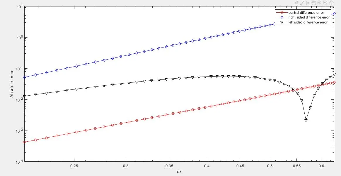
From the above graph, it can be stated that
- skewed right-sided difference approximation has the highest error and central difference approximation has the least error. so central difference approximation is more useful in most of the cases because of its stability.
- But when it is required to calculate error at the boundary, skewed left-sided or skewed right-sided difference approximation is more useful as compared to central difference approximation.
- Forward and backward difference approximation is also useful at the boundary, but it has higher error as compared to skewed systems.