Solving steady-state and unsteady state (Implicit and Explicit) 2D heat conduction equation using MATLAB
# Objective:
The objective of this project is to compare the convergence rate (Number of iterations) of the steady-state and transient simulation(Implicit and Explicit) of the 2D heat conduction equation solved by three iterative solvers like,
1) Jacobi
2) Gauss Seidel
3) SOR (successive over-relaxation)
# Problem Statement:
The problem statement and related assumptions taken in this project are,
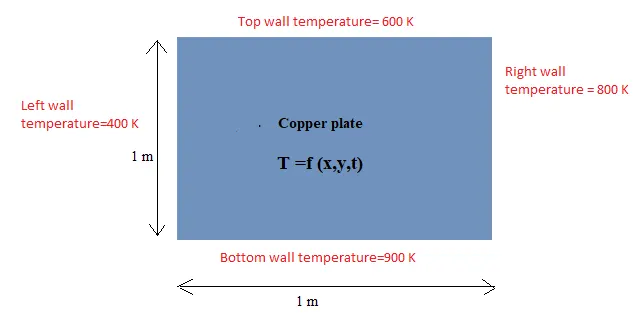
A copper Plate of 1x1 `m^2` is maintained at the temperature of 600 K at the top wall, 900 K at the bottom, 400 K at the left wall, and 800K at the right wall.
`alpha_(copper)=1.1times10^-4`
Nodes in x & y direction=10
Convergence criteria (tolerance)=1e-4
(1) Steady-State Heat Conduction:
Two-dimensional Steady-state heat conduction equation (without heat generation) can be written as,
`(del^2T)/(delx^2)+(del^2T)/(dely^2)=0`
To solve this equation numerically, it is required to discretize it with the central difference approximation method. after that, it can be written as,
`[(T_(i-1,j)-2*T_(i,j)+T_(i+1,j))/dx^2]+[(T_(i,j-1)-2*T_(i,j)+T_(i,j+1))/dy^2]`
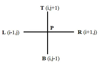
This equation can be rewritten using the above notation,
`T_P=1/K((T_L+T_R)/dx^2)+1/K((T_T+T_B)/dy^2)`
`K=2((dx^2+dy^2)/(dx^2*dy^2))`
# MATLAB Code:
This linear system of equations can be solved using different iterative solvers like Jacobi, Gauss seidel, and SOR.
In the Jacobi method, the previous iteration value is considered for the computation of the new value whereas in the Gauss Siedel method newly computed value is used in the same iteration.
In successive over-relaxation(SOR), relaxation factor(q) is used to compute the new value. here, q>1 is used for overrelaxation.
Input for the selection of the iterative solver is necessary for the execution of the 'if-else' loop in this below-attached MATLAB code.
Execution time is calculated using 'tic-toc' in MATLAB for the comparison of different methods.
close all
clear all
clc

%% steady state analysis of 2D heat conduction equation (d^2T/dx^2)+(d^2T/dy^2)=0

% inputs
nx=10;
ny=10;
x=linspace(0,1,nx);
y=linspace(0,1,ny);
dx=1/(nx-1);
dy=1/(ny-1);

% Defining temperature boundary condition and Initial guess value

T=ones(nx,ny);
T(1,2:nx-1)=600;
T(2:ny-1,1)=400;
T(end,2:nx-1)=900;
T(2:ny-1,end)=800;
T(1,1)=0.5*(T(1,2)+T(2,1));
T(1,end)=0.5*(T(1,nx-1)+T(2,end));
T(end,1)=0.5*(T(ny-1,1)+T(end,2));
T(end,end)=0.5*(T(end,nx-1)+T(ny-1,end));


K=2*((dx^2+dy^2)/(dx^2*dy^2));

[xx,yy]=meshgrid(x,y);

T_old=T;
error=100;
tol=1e-4;

%% input for Iterative solver

% [1] for jaccobi solver
% [2] for Guass Seidel solver
% [3] for SOR solver

iterative_solver=input('enter the desired number for itterative solver:');

 %% Jacobi solvers

 if iterative_solver==1
     tic;
     jacobi_iter=1;
         while (error>tol)
             for i=2:nx-1
                 for j=2:ny-1
                  T(i,j)=((T_old(i-1,j)+T_old(i+1,j))/(K*(dx^2)))+((T_old(i,j-1)+T_old(i,j+1))/(K*(dy^2)));
                 end
             end
          error=max(max(abs((T_old-T))));
          T_old=T;
          jacobi_iter=jacobi_iter+1;
         end
     time_J=toc;
     colormap(jet);
     [a,b]=contourf(xx,yy,T);
     colorbar
     xlabel('X');
     ylabel('Y');
     set(gca,'YDIR','reverse')
     clabel(a,b);
     title_text1=sprintf('For Steady State Analysis Jacobi Iteration Number=%d',jacobi_iter);
     title_text2=sprintf('execution time=%f',time_J);
     title({title_text1,title_text2})
 end

%% Gauss Siedel solvers

 if iterative_solver==2
     tic;
     GS_iter=1;
         while (error>tol)
             for i=2:nx-1
                 for  j=2:ny-1
                 T(i,j)=((T(i-1,j)+T_old(i+1,j))/(K*(dx^2)))+((T(i,j-1)+T_old(i,j+1))/(K*(dy^2)));
                 end
             end
          error=max(max(abs(T_old-T)));
          T_old=T;
          GS_iter=GS_iter+1;
         end
time_GS=toc;
colormap(jet);
[a,b]=contourf(xx,yy,T);
colorbar
xlabel('X');
ylabel('Y');
set(gca,'YDIR','reverse')
clabel(a,b);
title_text1=sprintf('For Steady State Analysis Gauss Seidel Iteration Number=%d',GS_iter);
title_text2=sprintf('execution time=%f',time_GS);
title({title_text1,title_text2})
 end


%% SOR( sucessive over relaxation) solver:

if iterative_solver==3
    tic;
    q=1.1;
    SOR_iter=1;
         while (error>tol)
             for i=2:nx-1
                 for  j=2:ny-1
                 T(i,j)=((1-q)*T_old(i,j))+(q*((T(i-1,j)+T(i+1,j))/(K*(dx^2)))+((T(i,j-1)+T(i,j+1))/(K*(dy^2))));
                 end
             end
          error=max(max(abs(T_old-T)));
          T_old=T;
          SOR_iter=SOR_iter+1;
         end
time_SOR=toc;
colormap(jet);
[a,b]=contourf(xx,yy,T);
colorbar
xlabel('X');
ylabel('Y');
set(gca,'YDIR','reverse')
clabel(a,b);
title_text1=sprintf('For Steady State Analysis SOR Iteration Number=%d',SOR_iter);
title_text2=sprintf('execution time=%f',time_SOR);
title({title_text1,title_text2})
 end
# Output:
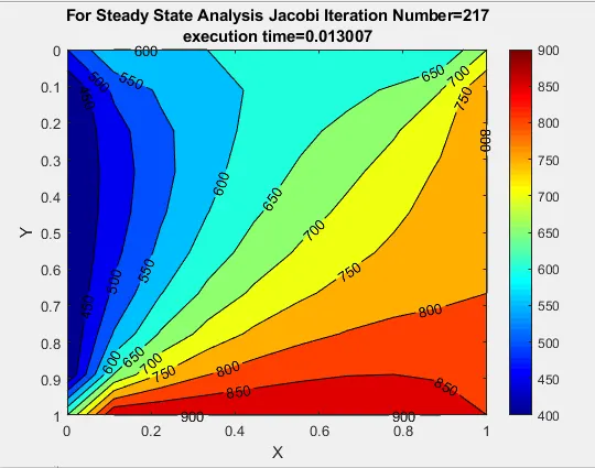
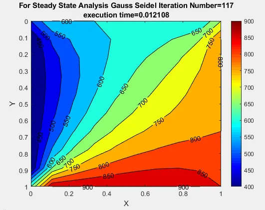
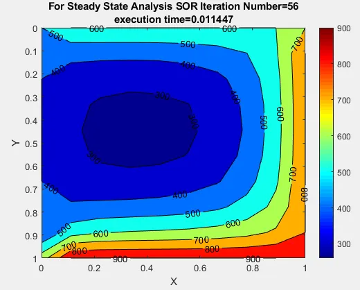
Numer of iteration and execution time for these three iterative solvers are,
| Steady-state | Jacobi | Gauss Siedel | SOR |
| Number of Iterations | 217 | 117 | 56 |
|
Execution time (in Seconds) |
0.0130 | 0.0121 | 0.0114 |
1)Jacobi:
2) Gauss-Seidel:
(3) SOR:
(2) Transient Heat Conduction:
Two-dimensional heat conduction equation for the transient state (without heat generation) can be written as,
`(del^2T)/(delx^2)+(del^2T)/(dely^2)=1/alpha*((delT)/(delt))`
where thermal diffusivity(`alpha`)=`K/(rho*C_p)`
To solve this equation, numerical discretization is required, and for that two different approaches like Implicit and Explicit Analysis are used.
(A) Explicit Analysis:
In the transient analysis, the nodal temperature generally changes for each time step. so to compute the above equation numerically central difference approximation is used for space derivative and forward difference approximation is used for time derivative.
In the case of explicit analysis, the temperature value of the previous time step(n) is used on the right-hand side of the equation to compute the temperature value of time step (n+1) on the left side of the equation.
`(T_(i,j)^(n+1)-T_(i,j)^n)/dt=alpha*[(T_(i-1,j)-2*T_(i,j)+T_(i+1,j))/dx^2+(T_(i,j-1)-2*T_(i,j)+T_(i,j+1))/dy^2]^n`
this equation can be rewritten as
`T_P^(n+1)=T_p^n+K_1(T_L-2*T_p+T_R)^n+K_2(T_T-2*T_P+T_B)^n`
`K_1=(alpha*dt)/dx^2`
`K_2=(alpha*dt)/dy^2`
# MATLAB Code:
The above equations can be solved using direct method. There is no need of iterative solvers and convergence criteria in Explicit method.
MATLAB code for Explicit method,
close all
clear
clc

%% Transient Analysis of 2D heat conduction equation dT/dt=alpha*(d^2T/dx^2)+(d^2T/dy^2) [Explicit Analysis]

% Inputs
nx=10;
ny=10;
alpha=1.1e-4;
dt=28;
nt=1000;
x=linspace(0,1,nx);
y=linspace(0,1,ny);
dx=1/(nx-1);
dy=1/(ny-1);

% Defining temperature boundary condition and Initial guess value

T=ones(nx,ny);
T(1,2:nx-1)=600;
T(2:ny-1,1)=400;
T(end,2:nx-1)=900;
T(2:ny-1,end)=800;
T(1,1)=0.5*(T(1,2)+T(2,1));
T(1,end)=0.5*(T(1,nx-1)+T(2,end));
T(end,1)=0.5*(T(ny-1,1)+T(end,2));
T(end,end)=0.5*(T(end,nx-1)+T(ny-1,end));

[xx,yy]=meshgrid(x,y);

T_old=T;
K1=(alpha*dt)/(dx^2);
K2=(alpha*dt)/(dy^2);

%% Direct solution explicit Analysis
tic;
for k=1:nt %time loop
    for i=2:nx-1   % space loop
        for j=2:ny-1
          term_1=(T_old(i-1,j)-2*T_old(i,j)+T_old(i+1,j));
          term_2=(T_old(i,j-1)-2*T_old(i,j)+T_old(i,j+1));
          T(i,j)=(T_old(i,j))+(K1*term_1)+(K2*term_2);
        end
    end
    T_old=T;
end
time=toc;
[a,b]=contourf(xx,yy,T);
colorbar
xlabel('X');
ylabel('Y');
set(gca,'YDIR','reverse')
clabel(a,b);
title_text1=sprintf('Explicit Transient Analysis time step=%d',k);
title_text2=sprintf('execution time=%f',time);
title({title_text1,title_text2})
# Output:
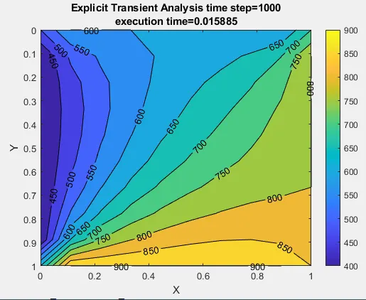
As there is no need for iterative solvers in the Explicit Method, it is easy to implement.
In the explicit analysis, it is required to satisfy the stability criteria which is defined by a dimensionless number called Mesh Fourier Number (CFL number).
Mesh Fourier Number should be less than or equal to 0.5 for the stability of the solution.
`alpha*dt(1/dx^2+1/dy^2)<=0.5`
from the above criteria, time step size (dt) can be calculated as the mesh size(dx & dy) value is known.
for the defined problem statement, the value of dt=28.
- The execution time required for 1000 iteration is 0.0158 seconds.
(B) Implicit Analysis:
In the case of Implicit analysis, the temperature value of the next time step(n+1) is used on the right-hand side of the equation to compute the temperature value on the left side of the equation. The implicit equation can be written as,
`(T_(i,j)^(n+1)-T_(i,j)^n)/dt=alpha*[(T_(i-1,j)-2*T_(i,j)+T_(i+1,j))/dx^2+(T_(i,j-1)-2*T_(i,j)+T_(i,j+1))/dy^2]^(n+1)`
The final equation of the implicit method can be derived from the above equation written as,
`T_P^(n+1)=1/(1+2K_1+2K_2)[T_P^n+K_1(T_L+T_R)^(n+1)+K_2(T_T+T_B)^(n+1)]`
# MATLAB code:
This linear system of equations can be solved using different iterative solvers like Jacobi, Gauss seidel, and SOR as described above.
To code the above transient equation in MATLAB, a time loop is required inside which convergence loop is being computed. For the simplification of the above equation term1,term2 and term3 is created inside the space loop.
Error is being calculated in each and every iteration inside the convergence loop by comparing the newly computed temperature value and old temperature value and if this error falls below the convergence criteria(1e-4) then the solution is being converged for a particular time step (T_previous). while execution of the convergence loop, the time step (T_previous) remains constant after that time step value will be updated.
Input for the selection of the iterative solver is necessary for the execution of the 'if-else' loop in this below-attached MATLAB code.
close all
clear
clc

%% Transient Analysis of 2D heat conduction equation dT/dt=alpha*(d^2T/dx^2)+(d^2T/dy^2) [Implicit Analysis]

% Inputs
nx=10;
ny=10;
alpha=1.1e-4;
dt=20;
nt=1000;
x=linspace(0,1,nx);
y=linspace(0,1,ny);
dx=1/(nx-1);
dy=1/(ny-1);

% Defining temperature boundary condition and Initial guess value

T=ones(nx,ny);
T(1,2:nx-1)=600;
T(2:ny-1,1)=400;
T(end,2:nx-1)=900;
T(2:ny-1,end)=800;
T(1,1)=0.5*(T(1,2)+T(2,1));
T(1,end)=0.5*(T(1,nx-1)+T(2,end));
T(end,1)=0.5*(T(ny-1,1)+T(end,2));
T(end,end)=0.5*(T(end,nx-1)+T(ny-1,end));

[xx,yy]=meshgrid(x,y);

T_old=T;
T_previous=T;

K1=(alpha*dt)/(dx^2);
K2=(alpha*dt)/(dy^2);

tol=1e-4;

%% input for Iterative solver

% [1] for jaccobi solver
% [2] for Guass Seidel solver
% [3] for SOR solver

iterative_solver=input('enter the desired number for itterative solver:');

%% jacobi solvers
 tic;
 if iterative_solver==1
  jacobi_iter=1;
        for k=1:nt
         error=9e9;
                while (error>tol)
                     for i=2:nx-1
                         for j=2:ny-1
                             term_1=1/(1+2*K1+2*K2);
                             term_2=K1*term_1;
                             term_3=K2*term_1;
                             H=T_old(i-1,j)+T_old(i+1,j);
                             V=T_old(i,j-1)+T_old(i,j+1);
                             T(i,j)=(term_1*T_previous(i,j))+(term_2*H)+(term_3*V);
                         end
                     end
                   error=max(max(abs((T_old-T))));
                   T_old=T;
                   jacobi_iter=jacobi_iter+1;
                 end
             T_previous=T;
        end
         J_time=toc;
         colormap(jet);
         [a,b]=contourf(xx,yy,T);
         colorbar
         xlabel('X');
         ylabel('Y');
         set(gca,'YDIR','reverse')
         clabel(a,b);
         title_text1=sprintf('Transient Implicit Analysis');
         title_text2=sprintf('Jacobi Iteration Number=%d',jacobi_iter);
         title_text3=sprintf('Execution time =%f',J_time);
         title({title_text1,title_text2,title_text3})
 end

%% Guass sediel solvers
 if iterative_solver==2
  tic;
  GS_iter=1;
        for k=1:nt
            error=9e9;
                  while (error>tol)
                     for i=2:nx-1
                         for j=2:ny-1
                             term_1=1/(1+2*K1+2*K2);
                             term_2=K1*term_1;
                             term_3=K2*term_1;
                             H=T(i-1,j)+T(i+1,j);
                             V=T(i,j-1)+T(i,j+1);
                             T(i,j)=(term_1*T_previous(i,j))+(term_2*H)+(term_3*V);

                         end
                     end
                          error=max(max(abs((T_old-T))));
                          T_old=T;
                          GS_iter=GS_iter+1;
                  end
             T_previous=T;
        end
        GS_time=toc;
        colormap(jet);
        [a,b]=contourf(xx,yy,T);
        colorbar
        xlabel('X');
        ylabel('Y');
        set(gca,'YDIR','reverse')
        clabel(a,b);
        title_text1=sprintf('Transient Implicit Analysis');
        title_text2=sprintf('Guass sediel Iteration Number=%d',GS_iter);
        title_text3=sprintf('Execution time =%f',GS_time);
        title({title_text1,title_text2,title_text3})
 end


%% SOR solvers
 if iterative_solver==3
  q=1.1;
  tic;
  SOR_iter=1;
        for k=1:nt
            error=9e9;
                  while (error>tol)
                     for i=2:nx-1
                         for j=2:ny-1
                             term_1=1/(1+2*K1+2*K2);
                             term_2=K1*term_1;
                             term_3=K2*term_1;
                             H=T(i-1,j)+T(i+1,j);
                             V=T(i,j-1)+T(i,j+1);
                             T(i,j)=((1-q)*T_old(i,j))+(q*(term_1*T_previous(i,j))+(term_2*H)+(term_3*V));

                         end
                     end
                               error=max(max(abs((T_old-T))));
                               T_old=T;
                               SOR_iter=SOR_iter+1;

                  end
             T_previous=T;

        end
             SOR_time=toc;
             colormap(jet);
             [a,b]=contourf(xx,yy,T);
             colorbar
             xlabel('X');
             ylabel('Y');
             set(gca,'YDIR','reverse')
             clabel(a,b);
             title_text1=sprintf('Transient Implicit Analysis');
             title_text2=sprintf('SOR iteration=%d',SOR_iter);
             title_text3=sprintf('Execution time =%f',SOR_time);
             title({title_text1,title_text2,title_text3})

 end
# Output:
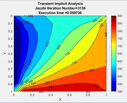
The implicit method is unconditionally stable so any time step can be used. The disadvantage of the implicit method is that it results in a set of equations that must be solved simultaneously for each time step. There is no need for stability criteria in the Implicit method but convergence criteria are required (1e-4).
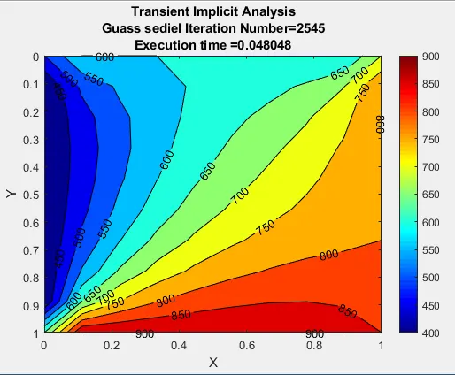
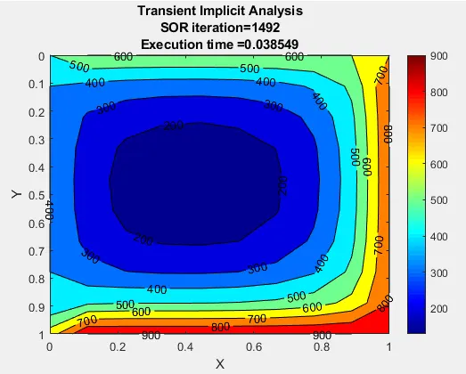
| Transient Analysis | Jacobi | Gauss-Seidel | SOR |
| Number of iterations | 3136 | 2545 | 1492 |
| Execution time(in seconds) | 0.0597 | 0.0480 | 0.0385 |
(1) Jacobi:
(2) Gauss-Seidel:
(3) SOR:
#Conclusion:
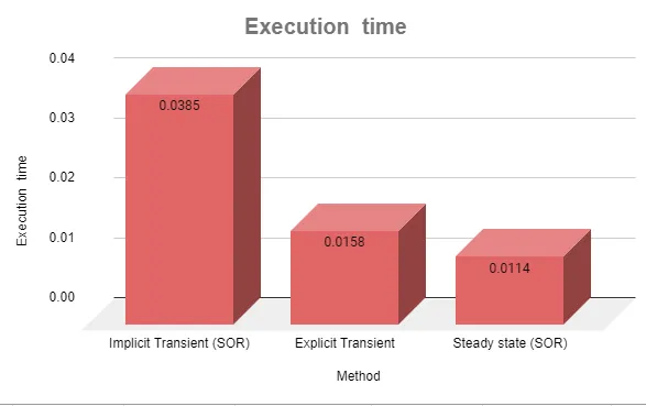
- The steady-state analysis takes less execution time as compared to transient analysis because it does not involve time loop iteration.
- Successive over-relaxation(SOR) requires the least number of iteration for convergence as compared to the other two iterative solvers.
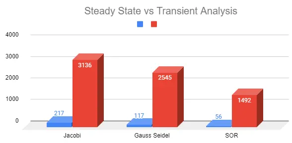
So, the number of iteration required in steady-state is less as compared to transient implicit analysis.
- In Transient analysis, explicit and implicit methods are used for the solution. one method is not necessarily better than the other one. Both the methods are practically used as per its own advantages and disadvantages.
- The explicit method requires less number of iteration and execution time as compared to the Implicit method. But the explicit method imposes a limit on the allowable time step to avoid the instabilities in the solution.
- The implicit method can be used for any time step condition as it does not involve any stability criteria but it takes a longer time for execution.