Simulation of a 1D Super-Sonic Nozzle Flow using MacCormack's Method in MATLAB
# Objective:
The objective of this project is to simulate the isentropic flow through a quasi 1D subsonic-supersonic nozzle. To derive the conservation and non-conservation forms of governing equation and solve them using MacCormack's technique.
# Problem Statement:
The physical problem of isentropic subsonic-supersonic flow can be solved using the analytical method. Here the aim is to solve this problem using Maccormack's method for conservation and nonconservation form and compare them with the exact analytical solution.
Assumption:
(1) Flow properties are uniform across any cross-section.
(2) Steady and isentropic flow.
(3) Flow is one dimensional (flow properties varies only with x)
(4) Area of the nozzle is a function of x.
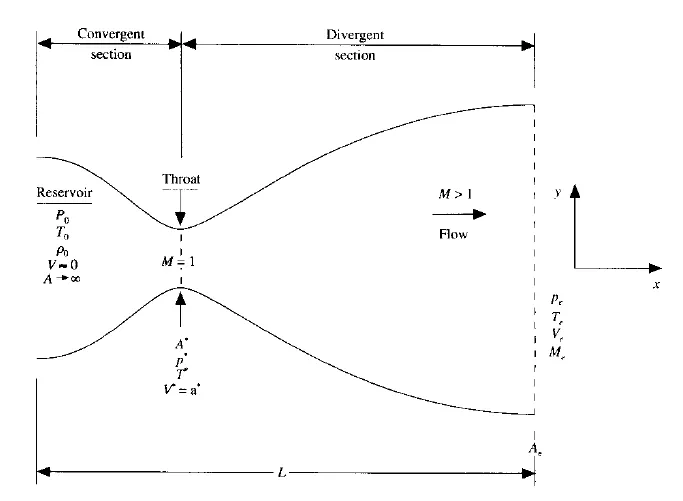
Analytical solution for all primitive variables given by,
`(A/A^**)^2=1/M^2[2/(gamma+1)(1+(gamma-1)/2*M^2)]^((gamma+1)/(gamma-1))`
`P/P^**=(1+(gamma-1)/2*M^2)^(-gamma/(gamma-1))`
`rho/rho^**=(1+(gamma-1)/2*M^2)^(-1/(gamma-1))`
`T/T^**=(1+(gamma-1)/2*M^2)^-1`
(* properties defines at the throat)
Governing equations:
The governing equations that describe the fluid flow can be obtained in various different forms based on two approaches,
(1) Finite control volume ( Integral form of governing equations)
(2) Infinitesimal fluid element approach (Partial differential form)
If the Finite control volume or Infinitesimal fluid element is fixed in space, then the equations derived (Either in integral or in a differential form) is known as conservation Form.
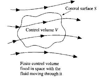
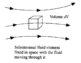
and If the Finite control volume or Infinitesimal fluid element is moving the fluid element, then the equations derived (Either in integral or in a differential form) is known as Non-conservation Form.
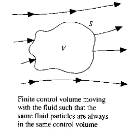
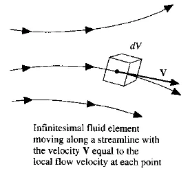
# Non-conservation Form:
The partial differential form of governing flow equations (which are suitable for the time marching solution in the MacCormack method) is used in the nonconservation form.
The non-dimensional form of equations can be represented as,
Continuity Equation:
`(delrho')/(delt)=-rho'((delv')/(delt))-rho'*v'((del(lnA'))/(delx'))-v'((delrho')/(delx'))`
Momentum Equation:
`(delv')/(delt)=-v'*((delv')/(delx'))-1/gamma*((delT')/(delx')+(T')/(rho')(delrho')/(delx'))`
Energy equation:
`(delT')/(delt)=-v'((delT')/(delx'))-(gamma-1)T'((delv')/(delx')+v'(del(lnA'))/(delx'))`
Initial Condition:
`rho=1-0.3146*x`
`T=1-0.2314*x`
`v=(0.1+1.09*x)T^(1/2)`
`A=1+2.2(x-1.5)^2` for `0<=x<=3`
x is divided into n number of grid points. and each and every grid point primitive variables are calculated using MacCormack's method. In MacCormack's Method time marching is done using predictor and corrector step.
Predictor Step:
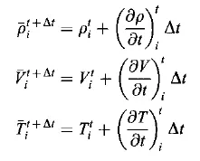
In this step, all the above equations are discretized with Forward difference scheme, and time derivative of primitive variables are calculated,



this time derivative is used to update all variables which are useful in the corrector step,
Corrector Step:
In this step, discretization is done using the Backward Difference scheme. After that average time derivative of all primitive variables are calculated,
`((delrho)/(delt))_(avg)=0.5[((delrho)/(delt))_p+((delrho)/(delt))_c]`
`((delv)/(delt))_(avg)=0.5[((delv)/(delt))_p+((delv)/(delt))_c]`
`((delT)/(delt))_(avg)=0.5[((delT)/(delt))_p+((delT)/(delt))_c]`
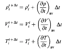
Final Solution updated:
Calculation of time step:
The Courant number is used for the stability criteria. Courant number(C) must be less than 1 to satisfy the stability criteria. from that dt can be calculated as,
`dt=C*dx/(T^(1/2)+v)`
dt has been calculated for all grid points (i=1 to i=N) using the above formula.
and at final,
dt=minimum(dt(1),dt(2),dt(3),...,dt(n))
Boundary Conditions:
- Inlet Boundary Condition:
At inlet flow is subsonic. Two variables (density and temperature) are fixed and one variable(velocity) is allowed to float at the inlet.
To calculate the velocity at the inlet, linear interpolation is used.
v(1)=2*v(2)-v(3)
- Outlet Boundary Condition:
At outlet flow is supersonic. All variables are allowed to float and linear interpolation is used to calculate the parameters at the outlet.
`rho(n)=2*rho(n-1)-rho(n-2)`
`v(n)=2*v(n-1)-v(n-2)`
`T(n)=2*T(n-1)-T(n-2)`
MATLAB Function:
The above mentioned MacCormack's method is coded in user-defined MATLAB function with the boundary condition. This function takes inputs like the number of grid point (n), a number of time steps (nt), throat value(which can be calculated using n). so, that this function can be called in the main MATLAB program to compare the different results.
function [rho,v,T,Ma,P,m,rho_th,v_th,T_th,Ma_th,m_th,P_th]=non_conservative(n,nt,throat)

    % inputs
    x=linspace(0,3,n);
    dx=x(2)-x(1);

    % Calculation of initial profile
    rho=1-0.3146*x;               %density profile
    T=1-0.2314*x;                 %Temperature profile
    v=(0.1+1.09*x).*T.^0.5;       % velocity profile
    a=1+2.2*(x-1.5).^2;           %area

    c=0.5;   %CFL criteria
    gamma=1.4;

  % calculation of time step
    for i=1:n-1
     dt_step(i)=c*(dx*(((T(i)^0.5)+v(i))^-1));
     dt=min(dt_step);
    end

   % time loop
    for k=1:nt
        rho_old=rho;
        v_old=v;
        T_old=T;

      % predictor loop
        for i=2:n-1

           drho_dx=((rho(i+1)-rho(i)))/dx;
           da_dx=(log(a(i+1))-log(a(i)))/dx;
           dv_dx=(v(i+1)-v(i))/dx;
           dT_dx=(T(i+1)-T(i))/dx;

           % continuty equation
           drho_dt_p(i)=-rho(i)*dv_dx-rho(i)*v(i)*da_dx-v(i)*drho_dx;

           %momentum equation
           dv_dt_p(i)=-v(i)*dv_dx-(1/gamma)*(dT_dx+(T(i)/rho(i))*drho_dx);

           % energy equation
           dT_dt_p(i)=-(v(i)*dT_dx)-((gamma-1)*T(i)*(dv_dx+v(i)*da_dx));

          % update solution
          rho(i)=rho(i)+drho_dt_p(i)*dt;
          v(i)=v(i)+dv_dt_p(i)*dt;
          T(i)=T(i)+dT_dt_p(i)*dt;

        end
        % corrector loop
        for j=2:n-1

           drho_dx=((rho(j)-rho(j-1)))/dx;
           da_dx=(log(a(j))-log(a(j-1)))/dx;
           dv_dx=(v(j)-v(j-1))/dx;
           dT_dx=(T(j)-T(j-1))/dx;


           % continuty equation
           drho_dt_c(j)=-rho(j)*dv_dx-rho(j)*v(j)*da_dx-v(j)*drho_dx;

           %momentum equation
           dv_dt_c(j)=-v(j)*dv_dx-(1/gamma)*(dT_dx+(T(j)/rho(j))*drho_dx);

           % energy equation
           dT_dt_c(j)=-(v(j)*dT_dx)-((gamma-1)*T(j)*(dv_dx+v(j)*da_dx));
        end
         % compute average time derivative
           drho_dt=0.5*(drho_dt_p+drho_dt_c);
           dv_dt=0.5*(dv_dt_p+dv_dt_c);
           dT_dt=0.5*(dT_dt_p+dT_dt_c);

       % update the solution
        for h=2:n-1
            rho(h)=rho_old(h)+drho_dt(h)*dt;
            v(h)=v_old(h)+dv_dt(h)*dt;
            T(h)=T_old(h)+dT_dt(h)*dt;
        end

        P=rho.*T;
        Ma=v.*(T.^-0.5);
        m=rho.*a.*v;

        % apply the boundary condition
        % Inlet
        v(1)=2*v(2)-v(3);

        %outlet
        rho(n)=2*rho(n-1)-rho(n-2);
        v(n)=2*v(n-1)-v(n-2);
        T(n)=2*T(n-1)-T(n-2);

    % storing the primitve variables at throat
     rho_th(k)=rho(throat);
     v_th(k)=v(throat);
     T_th(k)=T(throat);
     Ma_th(k)=Ma(throat);
     m_th(k)=m(throat);
     P_th(k)=P(throat);

   % variation of mass flow rate at different time steps during time marching
    figure(1)
    if k==50
        plot(x,m,'linewidth',1.5);
        hold on
    elseif k==100
        plot(x,m,'linewidth',1.5);
    elseif k==150
        plot(x,m,'linewidth',1.5);
    elseif k==200
        plot(x,m,'linewidth',1.5);
    elseif k==700
        plot(x,m,'linewidth',1.5);
        hold off

    grid on;
    xlabel('Nondimensional distance through nazeel(x)')
    ylabel('Nondimensional mass flow rate')
    legend({'dt=50','dt=100','dt=150','dt=200','dt=700'})
    title('Variation of mass flow rate for different time step(Nonconservative form)','color','r')
    end
    end
end
Output:
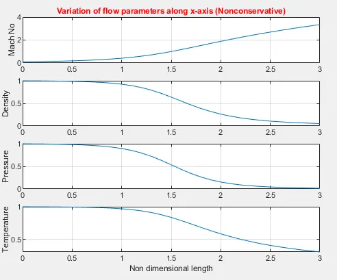
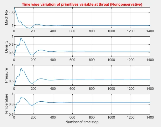
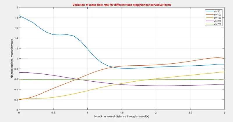
Different plots that describe the variation of primitive variables in the nonconservative form are plotted in the main MATLAB program. but it is attached below for a better understanding.
The value of the number of grid points (n=31) and timestep (nt=1400) is taken to reach a steady-state solution.
(1) Steady-state distribution of primitive variables inside the nozzle:
(2) Time wise variation of the primitive variables:
(3) Variation of mass flow rate at different time steps during the time marching process
# Conservation Form:
The basic governing equations in conservation form (Non-dimensional),
Continuity Equation:
`(del(rho'A'))/(delt)+(del(rho'A'v'))/(delx')=0`
Momentum equation:
Energy equation:

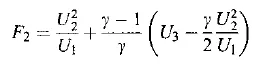
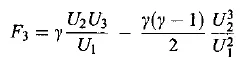
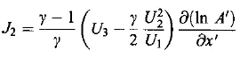
Defining the elements of the solution vector U, flux vector F, and source term J as
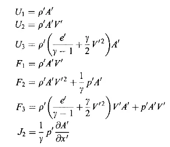
The governing equations can be rewritten using the above term,
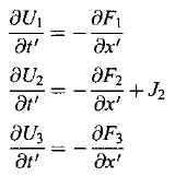
Primitive Variables must be decoded from the solution vector U1, U2, U3
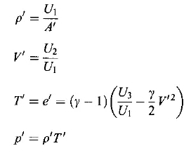
For the ease of CFD coding flux terms represented in the form of solution vector U.

Initial Condition:
for `0<=x'<=0.5`
`rho'=1`
`T'=1`
for `0.5<=x'<=1.5`
`rho'=1-0.366(x'-0.5)`
`T'=1-0.167(x'-0.5)`
for `1.5<=x'<=3.5`
`rho'=0.634-0.3679(x'-1.5)`
`T'=0.833-0.3507(x'-1.5)`
U2=0.590
`v'=0.59/(rho'*A')`
The Initial condition for Solution vector can be calculated using above primitive variables,
`U_1=rho'*A'`
`U_2=rho'*A'*v'`
`U_3=rho'((T')/(gamma-1)+gamma/2*v'^2)A'`
Boundary Condition:
- Inlet Condition:
Two variables are taken as fixed and one variable(velocity) is allowed to float.
`rho(1)=1`
T(1)=1
U1=`rho'*A'`=fixed
`U_2(1)=2*U_2(2)-U_2(3)`
form the above equation v can be decoded and it is used to calculate the U3.
- Outlet Condition:
The primitive variables and solution vector can be calculated using the linear interpolation method as mentioned in the non-conservation form.
The time step calculation and implementation of MacCormack's Method are the same as in the nonconservation form.
MATLAB function:
The above mentioned MacCormack's method is coded in user-defined MATLAB function with the boundary condition. This function takes inputs like the number of grid point (n), a number of time steps (nt), throat value(which can be calculated using n). so, that this function can be called in the main MATLAB program to compare the different results.
function [rho_c,v_c,T_c,Ma_c,P_c,m_c,rhoc_th,vc_th,Tc_th,Mac_th,mc_th,Pc_th]=conservartive(n,nt,throat)

% inputs
x=linspace(0,3,n);
dx=x(2)-x(1);

%% Intial conditions(t=0)

gamma=1.4;
a=1+2.2*(x-1.5).^2;   %area

for i=1:n
    if  (x(i)>=0 && x(i)<=0.5)
       rho_c(i)=1;
       T_c(i)=1;
    elseif (x(i)>=0.5 && x(i)<=1.5)
        rho_c(i)=1-(0.366*(x(i)-0.5));
        T_c(i)=1-(0.167*(x(i)-0.5));
    elseif (x(i)>=1.5 && x(i)<=3.5)
        rho_c(i)=0.634-(0.3879*(x(i)-1.5));
        T_c(i)=0.833-(0.3507*(x(i)-1.5));
    end
end

u1=rho_c.*a;
u2=0.590*ones(1,n);
v_c=u2.*(u1.^-1);
u3=rho_c.*((T_c.*((gamma-1)^-1))+((gamma/2)*(v_c.^2))).*a;

c=0.5; % CFL criteria

% Time step calculation
for i=1:n-1
 dt_step(i)=c*(dx*(((T_c(i)^0.5)+v_c(i))^-1));
 dt=min(dt_step);
end


%% MacCormack's explicit predictor-corrector Method

% Time loop
for k=1:nt
    rho_old=rho_c;
    v_old=v_c;
    T_old=T_c;
    u1_old=u1;
    u2_old=u2;
    u3_old=u3;

    f1=u2;
    f2=(u2.^2.*(u1.^-1))+((gamma-1)*(gamma^-1))*(u3-((gamma/2)*(u2.^2.*(u1.^-1))));
    f3=((gamma*u2.*u3).*(u1.^-1))-((0.5*gamma*(gamma-1))*(u2.^3).*(u1.^-2));

  % predicotr step
    for j=2:n-1

        da_dx=(log(a(j+1))-log(a(j)))/dx;
        J(j)=((gamma-1)*(gamma^-1))*(u3(j)-(0.5*gamma*u2(j)^2*(u1(j)^-1)))*(da_dx);

        % continuty
        du1_dt_p(j)=-(f1(j+1)-f1(j))/dx;
        % Momentum
        du2_dt_p(j)=-((f2(j+1)-f2(j))/dx)+J(j);
        % Energy
        du3_dt_p(j)=-((f3(j+1)-f3(j))/dx);

        % update solution
        u1(j)=u1(j)+du1_dt_p(j)*dt;
        u2(j)=u2(j)+du2_dt_p(j)*dt;
        u3(j)=u3(j)+du3_dt_p(j)*dt;

        f1(j)=u2(j);
        f2(j)=(u2(j)^2*(u1(j)^-1))+((gamma-1)*(gamma^-1))*(u3(j)-((gamma/2)*(u2(j)^2*(u1(j)^-1))));
        f3(j)=((gamma*u2(j)*u3(j))*(u1(j)^-1))-((0.5*gamma*(gamma-1))*(u2(j)^3).*(u1(j)^-2));

        % decoding the premitive variables
        rho_c(j)=u1(j)*(a(j)^-1);
        v_c(j)=u2(j)*(u1(j)^-1);
        T_c(j)=(gamma-1)*((u3(j)*(u1(j)^-1))-(0.5*gamma*(v_c(j)^2)));

    end

    %% corrector step
    for q=2:n-1
        da_dx_c=(log(a(q))-log(a(q-1)))/dx;
        J_c(q)=((gamma-1)*(gamma^-1))*(u3(q)-(0.5*gamma*u2(q)^2*(u1(q)^-1)))*(da_dx_c);

        % continuty
        du1_dt_c(q)=-(f1(q)-f1(q-1))/dx;
        % Momentum
        du2_dt_c(q)=-((f2(q)-f2(q-1))/dx)+J_c(q);
        % Energy
        du3_dt_c(q)=-((f3(q)-f3(q-1))/dx);

    end

 %% compute average time derivative

    du1_dt=0.5*(du1_dt_p+du1_dt_c);
    du2_dt=0.5*(du2_dt_p+du2_dt_c);
    du3_dt=0.5*(du3_dt_p+du3_dt_c);

 %% final solution update
 for e=2:n-1
    u1(e)=u1_old(e)+du1_dt(e)*dt;
    u2(e)=u2_old(e)+du2_dt(e)*dt;
    u3(e)=u3_old(e)+du3_dt(e)*dt;

    rho_c(e)=u1(e)*(a(e)^-1);
    v_c(e)=u2(e)*(u1(e)^-1);
    T_c(e)=(gamma-1)*((u3(e)*(u1(e)^-1))-(0.5*gamma*(v_c(e)^2)));
 end

 P_c=rho_c.*T_c;
 Ma_c=v_c.*(T_c.^-0.5);
 m_c=rho_c.*a.*v_c;

%% Boundary Conditions

% Inlet B.C
rho_c(1)=1;
T_c(1)=1;
u1(1)=rho_c(1)*a(1);
u2(1)=2*u2(2)-u2(3);
v_c(1)=u2(1)/u1(1);
u3(1)=u1(1)*((T_c(1)/(gamma-1))+((gamma/2)*v_c(1)^2));

% Outlet B.C
u1(n)=2*(u1(n-1))-u1(n-2);
u2(n)=2*(u2(n-1))-u2(n-2);
u3(n)=2*(u3(n-1))-u3(n-2);

rho_c(n)=u1(n)*(a(n)^-1);
v_c(n)=u2(n)*(u1(n)^-1);
T_c(n)=(gamma-1)*((u3(n)*(u1(n)^-1))-(0.5*gamma*(v_c(n)^2)));

    % storing the primitve variables at throat
     rhoc_th(k)=rho_c(throat);
     vc_th(k)=v_c(throat);
     Tc_th(k)=T_c(throat);
     Mac_th(k)=Ma_c(throat);
     mc_th(k)=m_c(throat);
     Pc_th(k)=P_c(throat);

% variation of mass flow rate at different time steps during time marching
    figure(2)
    if k==50
        plot(x,m_c,'linewidth',1.5);
        hold on
    elseif k==100
        plot(x,m_c,'linewidth',1.5);
    elseif k==150
        plot(x,m_c,'linewidth',1.5);
    elseif k==200
        plot(x,m_c,'linewidth',1.5);
    elseif k==700
        plot(x,m_c,'linewidth',1.5);
        hold off

    grid on;
    xlabel('Nondimensional distance through nazeel(x)')
    ylabel('Nondimensional mass flow rate')
    title('Variation of mass flow rate for different time step(conservative form)','color','r')
    legend({'dt=50','dt=100','dt=150','dt=200','dt=700'})

    end

end
end
Output:
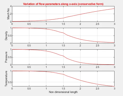
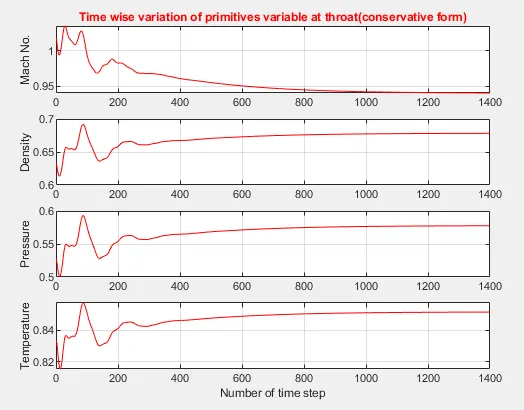
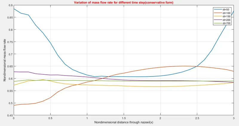
Different plots that describe the variation of primitive variables in the conservation form are plotted in the main MATLAB program. but it is attached below for a better understanding.
The value of the number of grid points (n=31) and timestep (nt=1400) is taken to reach a steady-state solution.
(1) Steady-state distribution of primitive variables inside the nozzle:
(2) Time wise variation of the primitive variables:
(3) Variation of mass flow rate at different time steps during the time marching process
# Main MATLAB Program:
close all
clear all
clc

n=31;
x=linspace(0,3,n);
dx=x(2)-x(1);
throat=((n-1)/2)+1;
nt=1400;
gamma=1.4;
m_analytical=0.579*ones(1,n);

%% non conservative form
[rho,v,T,Ma,P,m,rho_th,v_th,T_th,Ma_th,m_th,P_th]=non_conservative(n,nt,throat);

% Time wise variation of primitive variables at throat
figure(3)
subplot(4,1,1)
plot(linspace(1,nt,nt),Ma_th)
grid on;
title('Time wise variation of primitives variable at throat (Nonconservative)','color','r')
ylabel('Mach No')
subplot(4,1,2)
plot(linspace(1,nt,nt),rho_th)
grid on;
ylabel('Density')
subplot(4,1,3)
plot(linspace(1,nt,nt),P_th)
grid on;
ylabel('Pressure')
subplot(4,1,4)
plot(linspace(1,nt,nt),T_th)
grid on;
ylabel('Temperature')
xlabel('Number of time step')

% Steady-state variation of primitive variables inside the nozzle

figure(4)
subplot(4,1,1)
plot(x,Ma)
grid on;
title('Variation of flow parameters along x-axis (Nonconservative)','color','r');
ylabel('Mach No')
subplot(4,1,2)
plot(x,rho)
grid on;
ylabel('Density')
subplot(4,1,3)
plot(x,P)
grid on;
ylabel('Pressure')
subplot(4,1,4)
plot(x,T)
grid on;
ylabel('Temperature')
xlabel('Non dimensional length')

%% conservative form
[rho_c,v_c,T_c,Ma_c,P_c,m_c,rhoc_th,vc_th,Tc_th,Mac_th,mc_th,Pc_th]=conservartive(n,nt,throat);

%Time wise variation of primitive variables at throat
figure(5)
subplot(4,1,1)
plot(linspace(1,nt,nt),Mac_th,'color','r')
grid on;
title('Time wise variation of primitives variable at throat(conservative form)','color','r')

ylabel('Mach No.')
subplot(4,1,2)
plot(linspace(1,nt,nt),rhoc_th,'color','r')
grid on;
ylabel('Density')
subplot(4,1,3)
plot(linspace(1,nt,nt),Pc_th,'color','r')
grid on;
ylabel('Pressure')
subplot(4,1,4)
plot(linspace(1,nt,nt),Tc_th,'color','r')
grid on;
ylabel('Temperature')
xlabel('Number of time step')

figure(6)
subplot(4,1,1)
plot(x,Ma_c,'color','r')
grid on;
title('Variation of flow parameters along x-axis (conservative form)','color','r');
ylabel('Mach No')
subplot(4,1,2)
plot(x,rho_c,'color','r')
grid on;
ylabel('Density')
subplot(4,1,3)
plot(x,P_c,'color','r')
grid on;
ylabel('Pressure')
subplot(4,1,4)
plot(x,T_c,'color','r')
grid on;
ylabel('Temperature')
xlabel('Non dimensional length')


%% Comparision of Normalized mass flow rate distrribution of both the form
figure(7)
plot(x,m,'color','b','linewidth',1.5);
hold on
plot(x,m_c,'color','r','linewidth',1.5)
hold on
plot(x,m_analytical,'y','linewidth',1.5)
xlabel('Non-dimensional distance throught nozzel(x)')
ylabel('Non-dimensional mass flow rate')
legend({'Nonconservative form','conservative form','Exact Analytical Solution'})
# Grid Independence:
When a CFD problem is solved, initially it is a function of the number of grid points. flow variables continuously change as the number of grid points increases, because dx is going to decrease. After a continuous increase in the number of grid points, a point is reached where flow variables are no longer sensitive to the number of grid points.
In the above main program, the Grid Independence test is done to see the effect on the flow parameters.
Variation of parameters at the throat of the nozzle
|
Non-dimensional parameters |
Non-conservation (n=31) |
Non-conservation (n=61) |
conservation (n=31) |
conservation (n=61) |
Exact Analytical solution |
| `rho'` | 0.6387 | 0.6377 | 0.6783 | 0.6394 | 0.634 |
| T' | 0.8365 | 0.8354 | 0.8516 | 0.8350 | 0.833 |
| P' | 0.5342 | 0.5327 | 0.5777 | 0.5339 | 0.528 |
| Mach No | 0.9994 | 0.9998 | 0.9405 | 0.9998 | 1 |
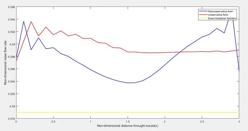
# Comparision of Normalized mass flow rate distribution of both the form:
The steady-state mass flow rate distribution predicted by the conservation form of the equations is much more satisfactory than the non-conservation form.
Conservation form gives distribution much closer to being constant whereas non-conservation form has sizable variation.
# Conclusion:
- The conservation form yields a better mass flow distribution. The conservation form simply does a better job of conserving mass.
- The amount by which residual decay is used as Quality of numerical algorithm. The non-conservation form leads to a smaller residual(`10^-6`) as compared conservation form(`10^-3`).
- The non-conservation form seems to produce slightly more accurate results for the primitive variables, and the conservation form seems to produce slightly more accurate results for flux variables.
- The solution of the conservation forms requires marginally more work because of the decoding of the primitive variables.