Week 9 - FVM Literature Review

# Finite Volume Method:

In the Finite Volume Method, discretization is based on an integral form of the partial differential equation (PDE) to be solved like conservation of mass, momentum, or energy. The PDE is written in a form that can be solved for a given finite volume. The computational domain is discretized into finite volumes and then for every volume, the governing equations are solved. The resulting system of equations usually involves fluxes of the conserved variable in FVM.

In the finite volume method, volume integrals in a partial differential equation that contain a divergence term are converted to surface integral, using Gauss Divergence Theorem.

`intintint(grad F)*dV=intint(F*n)dS`

# Difference between FDM and FVM:

FVM	FDM
The domain is divided into control volume or cells.	The domain is divided into the number of nodes.
Dependent variable values are stored at the centre of the cell (Volume).	Dependent variable values are stored at nodes only.
FVM can be easily formulated for unstructured mesh also.	FDM is formulated only for the structured mesh.
FVM is based on the integral form of the governing equations.	FDM is based on the differential form of the governing equations.
The Numerical schemes used in FVM is upwind differencing, Linear interpolation and TVD.	In FDM, Forward difference, backward difference and Central difference schemes are used.
It is difficult to accomplish higher-order schemes in FVM as compared to FDM.	It is difficult to handle geometrical complexity in FDM due to the requirement of the variable transformation technique.

# 1-D Linear Heat Conduction Equation:

For the understanding of FVM, 1-D Linear Heat Conduction with uniform heat generation is used.

`(del)/(delx)(k*(delT)/(delx))+S=0`

`int((del)/(delx)(k*(delT)/(delx))+S)dV=0`

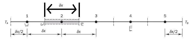
the highlighted portion represents the finite control volume and P denotes the centre of the control volume. The W and E are the center of the west and east side of the control volume.w and e represent the interface of the W-P and P-E respectively.

`int_w^e(del)/(delx)(k*(delT)/(delx))dV+intSdV=0`

In above equation dV=Adx , `intS*dV` represent the area under the curve.

`[k*(delT)/(delx)]_w^e+barS*dV=0`

`[(k*(delT)/(delx))_e-(k*(delT)/(delx))_w]+barsdV=0`

# Interpolaton Schemes:

Need for interpolation schemes:

The fundamental theorem used in the FVM is Gauss Divergence which converts the volume integral into the surface integral. The approximation of volume and surface integral may require the values of the variable at the location other than the nodes of the control volume. Values at this location are obtained using interpolation formulae.

There are various interpolation schemes are used like,

(1) First order Upwind Interpolation scheme:

In this method, We assume that the value at the interface is the same as the value at the centre of the control volume depending on the direction of the flow. results obtained from this method are stable but very diffusive.

`phi_e=phi_P` if flow direction is left to right.

`phi_e=phi_E` if flow direction is right to left

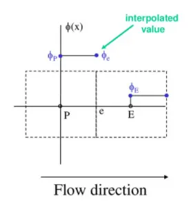
for the above heat conduction equation flow is assumed from left to right.

`phi_e=kA((T_E-T_P)/dx)`

(2) Linear Interpolation (CDS):

In Linear Interpolation (or central difference scheme), the value of flux(`phi`) can be determined by linear interpolation between the centres of the control volume.

This scheme is more accurate than the first-order upwind scheme but it leads to oscillations in the solution or divergence if the local peclet number is greater than 2.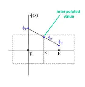

`phi_e=(phi_E+phi_P)/2`

(3) Second-Order Upwind Scheme:

In this method, the value of flux at the interface is determined from two points upstream of the direction of the flow.

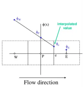
`phi_e=(3phi_P-phi_W)/2`

(4) Quadratic Upwind Interpolation for Convective Kinetics (QUICK) scheme :

In this method, two upstream centres and one downstream centre of the control volumes with the quadratic Interpolation is used.

This is a very accurate scheme but in regions with strong gradients, overshoot and undershoot can occur.

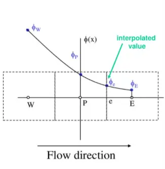
`phi_e=phi_P+(phi_E-phi_P)/2-(phi_E-2phi_P+phi_W)/8`

# Flux Limiters:

Flux Limites is used in a high-resolution scheme to avoid the spurious oscillations (wiggles) that would otherwise occur with high order spatial discretization schemes due to shocks, discontinuities or sharp changes in the solution domain.

The use of flux limiters, together with an appropriate high-resolution scheme, make the solutions Total variation diminishing (TVD).

The main idea behind the construction of flux limiter schemes is to limit the spatial derivatives to realistic values – for scientific and engineering problems this usually means physically realisable and meaningful values.

They are used in high-resolution scheme for solving problems described by PDEs and only come into operation when sharp wavefronts are present. For smoothly changing waves, the flux limiters do not operate and the spatial derivatives can be represented by higher-order approximations without introducing spurious oscillations.