Solution of 1-D Linear Convection equation using MATLAB and the effect of time step on stabillity of the solution

# Objective:

The objective is to solve the one-dimensional linear convection equation for the unit step velocity profile and to observe convection phenomena for the number of time steps.

and to study the effect of time step on linear convection phenomena.

Length of the domain=1 m

velocity profile: 2 m/s between 0.1 and 0.3 and 1 m/s for rest all value of x.

velocity constant (c)= 1

total time=0.4 sec

time step (dt)= 1e-4,1e-3,1e-2,1e-1

# Linear Convection Equation:

One dimensional linear convection equation can be written as,

`(delu)/(delt)+C*(delu)/(delx)=0`

To solve this one-dimensional partial derivative equation numerically, it is required to discretize the derivative terms.

so, first-order forward differencing is used for the time derivative and first-order backward differencing is used for the space derivative.

To solve this equation, explicit time integration is used in which the right-hand side of the equation is known.

`((u_2^(n+1)-u_2^n)/dt)+C*((u_2^n-u_1^n)/dx)=0`

This is used to calculate the velocity (u) at node 2 for `(n+1)^(th)`time step given that velocity at node 1 and node 2 is known for the `n^(th)`time step.

`u_2^(n+1)=u_2^n-((c*dt)/dx)[u_2^n-u_1^n]` ----(1)`

# Function Generation in MATLAB :

To solve the above equation no (1) for different values of time steps it is required to generate the function which can be called in MATLAB code whenever it is required.

so, to create a velocity profile from input data, first of all, the Length of the domain is divided into the required number of grid points (n).To get the length between each grid point,

`dx=L/(n-1)`

Now, to get the velocity profile which is having the value of 2 m/s between 0.1 to 0.3, it is required to represent it's in the function of the number of grid point(n).so that when n changes it takes the velocity profile in each and every iteration.

so here, the velocity profile is defined in three different intervals and the increasing value of x is function dx. where dx is represented in the function of n. so, velocity profile set up according to the number of grid points n.

Here, the MATLAB function called 'linear_convection' is created. which take input parameters such as length, no of grid points, total time, the velocity constant, and more importantly time step values. As an output, it generates the final velocity profile after solving the 1D linear convection equation numerically. for that one time loop and one space loop is used to create the final velocity profile.

function LC=linear_convection(l,n,c,t,dt)
%% velocity profile

dx=l/(n-1);
x1=0:dx:0.1;
x2=0.1:dx:0.3;
x3=0.3:dx:1;

x=[x1 x2 x3];

u=[1*ones(size(x1)) 2*ones(size(x2)) 1*ones(size(x3))];

u_old=u;
nt=t/dt; % no of time step 

%% Time Marching
    for k=1:nt    %Time loop  
        hold on
           for i=2:n   %space loop

             u(i)=u_old(i)-((c*dt/dx)*(u_old(i)-u_old(i-1)));

           end

          u_old=u;   %updating new value 
          LC=u;
    end

end

# MATLAB code:

The calculation of this 1D linear convection equation for different values of the 'dt' (time steps) is done in the main MATLAB code by calling the 'Linear_convection' function for the different values of the dt.

close all
clear all
clc
%% input variables

l=1;  %length of domain
n=80; % no of grid point 
c=1;     %velocity constant
t=0.4;  %total time
dt=[1e-4 1e-3 1e-2 1e-1];

dx=l/(n-1);
x1=0:dx:0.1;
x2=0.1:dx:0.3;
x3=0.3:dx:1;

x=[x1 x2 x3];
%% Calculation for different values dt

[LC_1]=linear_convection(l,n,c,t,dt(1));
[LC_2]=linear_convection(l,n,c,t,dt(2));
[LC_3]=linear_convection(l,n,c,t,dt(3));
[LC_4]=linear_convection(l,n,c,t,dt(4));

%% plotting the results and comparison of the output

figure(1)
axis([0 1 0 2]);
plot(x,LC_1,'b','linewidth',2)
hold on
plot(x,LC_2,'r','linewidth',2)
plot(x,LC_3,'y','linewidth',2)
plot(x,LC_4,'k','linewidth',2)
hold off

xlabel('X')
ylabel('velocity (u)')
legend(['dt= ',num2str(dt(1))],['dt= ',num2str(dt(2))],['dt= ',num2str(dt(3))],['dt= ',num2str(dt(4))])
title('Linear convection 1D euation for t=0.4 sec')

# Output:

comparison for different values of dt (time steps) can be done by plotting them in a single graph with a common axis.

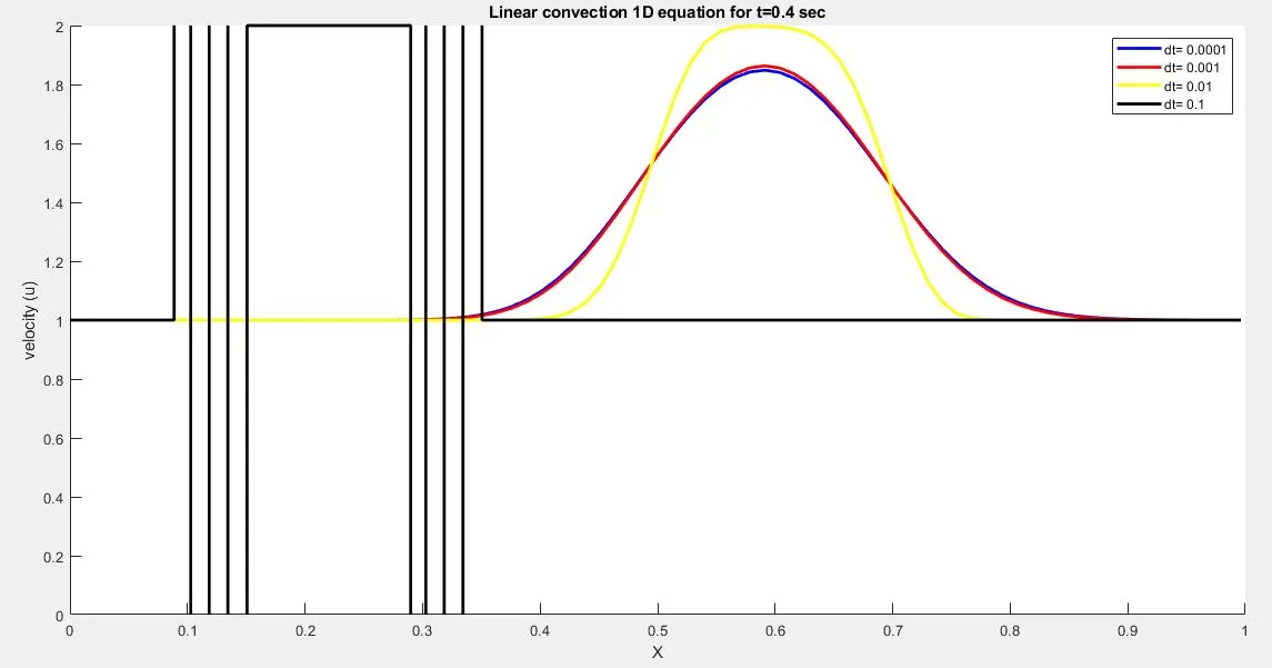
From the above graph, it can be stated that the solution for dt=0.1 unstable.

As the value of dt decreases the number of time steps to compute the solution is increased and as a result time required for computation is also increase.

For the dt=0.0001, it takes the maximum amount of time for the computation because it has the highest number of time steps to compute.