Week 3 - Taylor table method and Matlab code

Aim:

To Derive the following 4th order approximations of the second-order derivative with

1. Central difference

2. Skewed right-sided difference

3. Skewed left-sided difference

Introduction:

The no.of nodes used in the equations used for the 4th order approximation were derived from the p+q method.

Where p - order of derivation

q - order of approximation.

The no.of nodes in the central differencing scheme is p+q-1. Where as for the skewed left and right sided scheme the no.of nodes are p+q.

For the calculating the Skewed scheme we used Taylar's table. By writting the these table in the matrix multiplication form will find the unknown values.

1. Central difference scheme:

No.of nodes = 4+2-1 = 5

Formula for 'Central differencing scheme' is `(d^2u)/(dx^2) = (a*f(i-2)+b*f(i-1)+c*f(i)+d*f(i+1)+e*f(i-2))/(Deltax)`

By applying the Taylor's table method will get the values of (a,b,c,d,e,f).

Taylor's table for 'Central differencing scheme' is

	`f(i)`	`Deltax*f'(i)`	`Deltax^2*f''(i)`	`Deltax^3*f'''(i)`	`Deltax^4*f''''(i)`
`a*f(i-2)`	`a`	`-2a`	`(4a)/2`	`(-8a)/6`	`(16a)/24`
`b*f(i-1)`	`b`	`-b`	`b/2`	`-b/6`	`b/24`
`c*f(i)`	`c`	`0`	`0`	`0`	`0`
`d*f(i+1)`	`d`	`d`	`d/2`	`d/6`	`d/24`
`e*f(i+2)`	`e`	`2e`	`(4e)/2`	`(8e)/6`	`(16e)/24`
`Sum`	`0`	`0`	`1`	`0`	`0`

2. Skewed right-sided difference scheme:

No.of nodes = 4+2= 6

Formula for 'Skewed right-sided differencing scheme' is `(d^2u)/(dx^2) = (a*f(i)+b*f(i+1)+c*f(i+2)+d*f(i+3)+e*f(i+4)+g*f(i+5))/(Deltax)`

By applying the Taylor's table method will get the values of (a,b,c,d,e,f,g).

Taylor's table for 'Skewed right-sided differencing scheme' is

	`f(i)`	`Deltax*f'(i)`	`Deltax^2*f''(i)`	`Deltax^3*f'''(i)`	`Deltax^4*f''''(i)`	`Deltax^5*f'''''(i)`
`a*f(i)`	`a`	`0`	`0`	`0`	`0`	`0`
`b*f(i+1)`	`b`	`b`	`b/2`	`b/6`	`b/24`	`b/120`
`c*f(i+2)`	`c`	`2c`	`(4c)/2`	`(8c)/6`	`(16c)/24`	`(32c)/120`
`d*f(i+3)`	`d`	`3d`	`(9d)/2`	`(27d)/6`	`(81d)/24`	`(243d)/120`
`e*f(i+4)`	`e`	`4e`	`(16e)/2`	`(64e)/6`	`(256e)/24`	`(1024e)/120`
`g*f(i+5)`	`g`	`5g`	`(25g)/2`	`(125g)/6`	`(625g)/24`	`(3125g)/120`
`Sum`	`0`	`0`	`1`	`0`	`0`	`0`

3. Skewed left-sided difference scheme:

No.of nodes = 4+2= 6

Formula for 'Skewed left-sided differencing scheme' is `(d^2u)/(dx^2) = (a*f(i)+b*f(i-1)+c*f(i-2)+d*f(i-3)+e*f(i-4)+g*f(i-5))/(Deltax)`

By applying the Taylor's table method will get the values of (a,b,c,d,e,f,g).

Taylor's table for 'Skewed left-sided differencing scheme' is

	`f(i)`	`Deltax*f'(i)`	`Deltax^2*f''(i)`	`Deltax^3*f'''(i)`	`Deltax^4*f''''(i)`	`Deltax^5*f'''''(i)`
`a*f(i)`	`a`	`0`	`0`	`0`	`0`	`0`
`b*f(i+1)`	`b`	`-b`	`b/2`	`-b/6`	`b/24`	`-b/120`
`c*f(i+2)`	`c`	`-2c`	`(4c)/2`	`-(8c)/6`	`(16c)/24`	`-(32c)/120`
`d*f(i+3)`	`d`	`-3d`	`(9d)/2`	`-(27d)/6`	`(81d)/24`	`-(243d)/120`
`e*f(i+4)`	`e`	`-4e`	`(16e)/2`	`-(64e)/6`	`(256e)/24`	`-(1024e)/120`
`g*f(i+5)`	`g`	`-5g`	`(25g)/2`	`-(125g)/6`	`(625g)/24`	`-(3125g)/120`
`Sum`	`0`	`0`	`1`	`0`	`0`	`0`

By writting the these table in the matrix multiplication form will find the unknown values.

Matlab code:

clear all
close all
clc


x = (pi/3); 
dx = linspace(pi/4000,pi/40,20);
% Analytical function
K = exp(x)*cos(x);
% Analytical_function = exp(x)*cos(x);

% Analytical derivative
% f'(x) = exp(x)*cos(x)-exp(x)*sin(x);
% f"(x) = -2*exp(x)*sin(x);
Analytical_derivative =  -2*exp(x)*sin(x);
% sin (pi/3) = 0.8660
% cos(pi/3) = 0.5 

% Right sided difference scheme
A_R = [1 1 1 1 1 1; 0 1 2 3 4 5; 0 1/2 4/2 9/2 16/2 25/2; 0 1/6 8/6 27/6 64/6 125/6; 0 1/24 16/24 81/24 256/24 625/24; 0 1/120 32/120 243/120 1024/120 3125/120];
B_R = [0;0;1;0;0;0];
% A*B=X
% B_R = (X_R/A_R)
X = linsolve(A_R,B_R);

% Left sided difference scheme
A_L = [1 1 1 1 1 1; 0 -1 -2 -3 -4 -5; 0 1/2 4/2 9/2 16/2 25/2; 0 -1/6 -8/6 -27/6 -64/6 -125/6; 0 1/24 16/24 81/24 256/24 625/24; 0 -1/120 -32/120 -243/120 -1024/120 -3125/120];
B_L = [0; 0; 1; 0; 0; 0];
%B_L = (X_L./A_L)
Y = linsolve(A_L,B_L);

% Central difference scheme
A_C = [1 1 1 1 1; -2 -1 0 1 2; 4/2 1/2 0 1/2 4/2; -8/6 -1/6 0 1/6 8/6; 16/24 1/24 0 1/24 16/24];
B_C = [0; 0; 1; 0; 0];
% B_C = (X_C./A_C)
Z = linsolve(A_C,B_C);



% Numerical derivative 
for i= 1:length(dx)
% Central difference
Central_differencing(i) = (((-1/12)*exp(x-(2*dx(i)))*cos(x-(2*dx(i)))+(4/3)*exp(x-(dx(i)))*cos(x-(dx(i)))+(-5/2)*exp(x)*cos(x)+(4/3)*exp(x+(dx(i)))*cos(x+(dx(i)))-(1/12)*exp(x+(2*dx(i)))*cos(x+(2*dx(i))))/(dx(i)^2));

% Skewed right-sided difference
Skew_right_differencing(i) = (((15/4)*exp(x)*cos(x)+(-77/6)*exp(x+(dx(i)))*cos(x+(dx(i)))+(107/6)*exp(x+(2*dx(i)))*cos(x+(2*dx(i)))+(-13)*exp(x+(3*dx(i)))*cos(x+(3*dx(i)))+(61/12)*exp(x+(4*dx(i)))*cos(x+(4*dx(i)))+(-5/6)*exp(x+(5*dx(i)))*cos(x+(5*dx(i))))/(dx(i)^2));

% Skewed left-sided difference
Skew_left_differencing(i) =(((15/4)*exp(x)*cos(x)+(-77/6)*exp(x-(dx(i)))*cos(x-(dx(i)))+(107/6)*exp(x-(2*dx(i)))*cos(x-(2*dx(i)))+(-13)*exp(x-(3*dx(i)))*cos(x-(3*dx(i)))+(61/12)*exp(x-(4*dx(i)))*cos(x-(4*dx(i)))+(-5/6)*exp(x-(5*dx(i)))*cos(x-(5*dx(i))))/(dx(i)^2));

% Forward_differencing
%Forward_differencing = exp(x+dx(i))*cos(x+dx(i))+exp(x)*cos(x)

% Backward_differencing
%Backward_differencing = exp(x-dx(i))*cos(x-dx(i))+exp(x)*cos(x)
end


% Error calculation
Central_error = abs(Analytical_derivative - Central_differencing);
Skew_right_error = abs(Analytical_derivative - Skew_right_differencing);
Skew_left_error = abs(Analytical_derivative - Skew_left_differencing);

% Plotting
 figure(1)
 loglog(dx,Central_error,'marker','hexagram')
 hold on
 loglog(dx,Skew_right_error,'marker','s')
 hold on
 loglog(dx,Skew_left_error,'marker', 'o')
 grid on
 xlabel('dx')
 ylabel('error')
 legend('Central error','Skew right error','Skew left error') 
 
 

Procedure:

• Initially defined the x, dx and analytical function and then did analytical second order derivation.
• From the Taylor's table method extacted the unknowns of 4th order approximations of the second-order derivative for skewed right sided, skew left sided and central difference formulae.
• Then, applied those unknowns in the equation and solved.
• Then, caluclated the error difference between analytical derivative and skewed left, skew right & skew left scheme.
• Then, plotted the graph to observe the error difference.

Results:

• plot that compares the absolute error between the central, skew right & skew left errors:

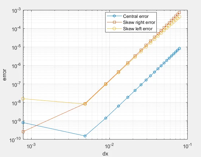
• Skew right error is higher than the skew left and central error.
• Skew left error is higher than central error and less than skew left error.
• Central difference error is smaller than the skewed left and skewed right errors.
• Till 10^-2 the central differencing error is smaller, but if we reduce further the errors are increasing gradually and the skewed right error is less at 10^-3 due to roundoff error.

Conclusion:

From the plot we can conclude that central differencing is smaller than skewed left and skewed right under certain limit, later it start increasing.

skewed scheme:

In this challenge, although central difference gives less error as compared to skewen right and left side difference, but in some cases skewed difference scheme is more useful as compaired to the cental difference scheme.

For example if we want to calcualte the error at the nodes closer to the boundaries, for computation will require higher order approximations. In such case we cannot use the central difference scheme since it require value from both the end. In this case we can apply skewed difference scheme.

Also, we can calculate the error at the boundry by using forward differencing or backward differencing scheme, but FDS and BDS has low order of approximation. So, it would be having more error. Therefore, skewed difference scheme is prefered in such case.