Aim:

To write a program that solves the following ODE in MATLAB.

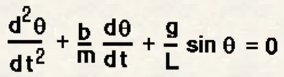
This ODE represents the equation of motion of a simple pendulum with damping.

In the above equation,

g = gravity in m/s2,

L = length of the pendulum in m,

m = mass of the ball in kg,

b=damping coefficient.

Objective:

1. Write a program in MATLAB that will simulate the pendulum motion.

use,

L=1 metre,

m=1 kg,

b=0.05.

g=9.81 m/s2.

2. Simulate the motion between 0-20 sec, for angular displacement=0, angular velocity=3 rad/sec at time t=0.
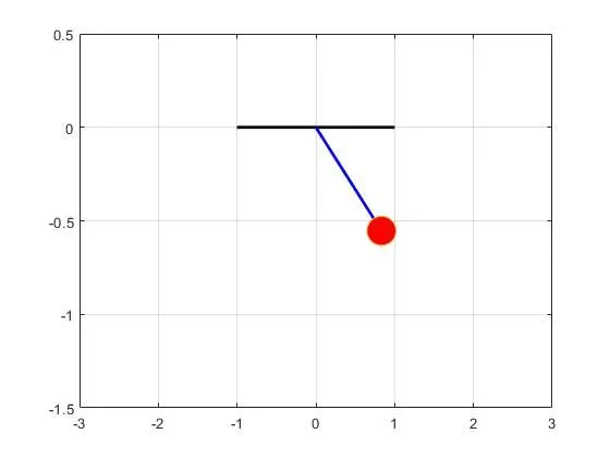
3. When you do this, you will get the position of the pendulum as a function of time. Use this information to animate the motion of the pendulum.

Programme Code to solve ODE:

clear all
close all
clc

L = 1; 
m = 1; 
b = 0.05;
g = 9.81;

% initial condition at theta = 0, 
% initial displacement = 0, initial velocity = 5 m/s.  
theta_0 = [0;3];

% to integrate ODE for the system we need time.
t_span = linspace(0,20,500);

%ODE syntax
[t, results] = ode45(@(t,theta) ode_func(t, theta, b, g, L, m), t_span, theta_0);

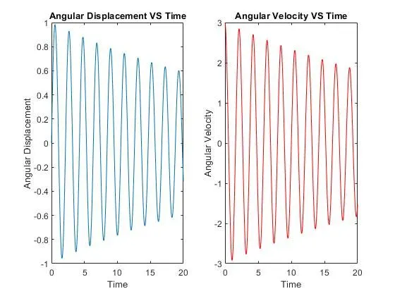
figure(1)

subplot(1,2,1)

plot(t,results(:,1))
xlabel('Time')
ylabel('Angular Displacement')
title('Angular Displacement VS Time')

subplot (1,2,2)

plot(t, results(:,2),'color','r')
xlabel('Time')
ylabel('Angular Velocity')
title('Angular Velocity VS Time')

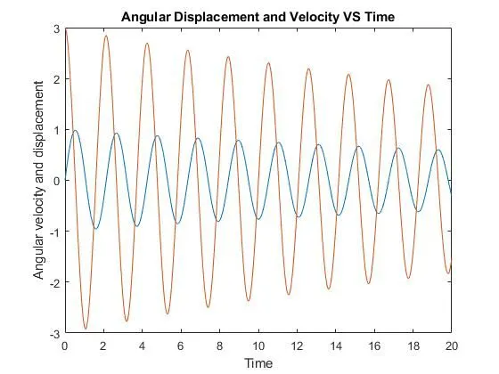
figure(2)

plot(t, results(:,1))
hold on 
plot(t, results(:,2))
xlabel('Time')
ylabel('Angular velocity and displacement') % Agnglar displacement is in radian.
title('Angular Displacement and Velocity VS Time')


% Animation of Pendulum

displacement = results(:,1);
ct = 1;
for i = 1 : length(displacement)
   theta = displacement(i);
   L = 1;
   x0  = 0;
   y0 = 0;
   x1 = L * sin(theta) % no "sind", since theta is in radian.
   y1 = -L * cos(theta)
   
   figure(3)
   
   plot([1 -1], [0 0],'linewidth' ,2,'color','k');
   hold on ;
   plot([x0 x1], [y0 y1], 'linewidth' ,2, 'color','b');
   plot(x1, y1, '-o','markers',20,'markerfacecolor','r');
   grid on
   hold off
   axis ([-3 3 -1.5 .5]);
   pause(0.03);
   
   M(ct) = getframe(gcf);
   ct = ct + 1;
end

movie(M)
videofile = VideoWriter('ode_Pendulum_motion.avi','uncompressed AVI');
open(videofile)
writeVideo(videofile,M)
close(videofile)

Function Code:

function [dtheta_dt] = ode_func(t,theta,b,g,L,m)

theta1 = theta(1)
theta2 = theta (2)

dtheta1_dt = theta2;
dtheta2_dt = -(b/m)*theta2 - (g/L)*sin(theta1);

%combining 2 ODEs into an array or a column matrix
dtheta_dt = [dtheta1_dt; dtheta2_dt];

end

Steps taken:

• Firstly, we need to break down higher order ODE into first order ODEs.

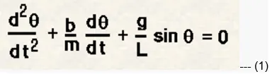
Since, --- (1)

is a second order ODE,

let θ = θ1

so dθ/dt = dθ1/dt = θ2 (say)

hence, (1) becomes

d θ2/dt + (b/m) θ2 + (g/L) sin θ1 = 0

now, we have two first order ODEs,

dθ1/dt = θ2

&

d θ2/dt = - (b/m) θ2 - (g/L) sin θ1

• Writing function code for ODE in MATLAB:

function [dtheta_dt] = ode_func(t,theta,b,g,L,m)

theta1 = theta(1)

theta2 = theta (2)

dtheta1_dt = theta2;

dtheta2_dt = -(b/m)*theta2 - (g/L)*sin(theta1);

%combining 2 ODEs into an array or a column matrix.

dtheta_dt = [dtheta1_dt; dtheta2_dt];

end

• Writting Programme code in MATLAB using ODE45 function for a simple pendulum:

clear all

close all

clc

L = 1;

m = 1;

b = 0.05;

g = 9.81;

% initial condition at theta = 0,

% initial displacement = 0, initial velocity = 5 m/s.

theta_0 = [0;3];

% To integrate ODE for the system we need time.

% following command will create 500 time intervals between 0-20seconds.

t_span = linspace(0,20,500);

% ODE syntax.

[t, results] = ode45(@(t,theta) ode_func(t, theta, b, g, L, m), t_span, theta_0);

% Writing codes to get plots.

figure(1)

subplot(1,2,1)

plot(t,results(:,1))

xlabel('Time')

ylabel('Angular Displacement')

title('Angular Displacement VS Time')

subplot (1,2,2)

plot(t, results(:,2),'color','r')

xlabel('Time')

ylabel('Angular Velocity')

title('Angular Velocity VS Time')

figure(2)

plot(t, results(:,1))

hold on

plot(t, results(:,2))

xlabel('Time')

ylabel('Angular velocity and displacement') % Agnglar displacement is in radian.

title('Angular Displacement and Velocity VS Time')

• Creating a pendulum animation plot:

%Here we are using "for loop" command to get the position of the mass/ball for all possible value of Angular Displacement.

%Angular Displacement is listed in "column one of the 'results' array"

% Here, Angular Displacement is in Radian and not Degree.

displacement = results(:,1);

ct = 1;

for i = 1 : length(displacement)

theta = displacement(i);

L = 1;

x0 = 0;

y0 = 0;

x1 = L * sin(theta)

y1 = -L * cos(theta)

figure(3)

plot([1 -1], [0 0],'linewidth' ,2,'color','k');

hold on ;

plot([x0 x1], [y0 y1], 'linewidth' ,2, 'color','b');

%Following command is used to create mass/ball.

plot(x1, y1, '-o','markers',20,'markerfacecolor','r');

grid on

hold off

axis ([-3 3 -1.5 .5]);

pause(0.03);

% 'getframe' command is used capture the frame for every value of counter. The frame obtained are assigned to 'M'.

M(ct) = getframe(gcf);

ct = ct + 1;

end

• Saving the pendulum animation as a video file:

% Creating video file using "VideoWriter" command and giving the file name as "ode_Pendulum_motion".

movie(M)

videofile = VideoWriter('ode_Pendulum_motion.avi','uncompressed AVI');

open(videofile)

writeVideo(videofile,M)

close(videofile)

Note:

• "%" is used to add comments in between codes.

• The Function Code should be saved in same directory and folder as the Programme code file.

• [t, results] = ode45(@(t,theta) ode_func(t, theta, b, g, L, m), t_span, theta_0);

In this ODE syntax

@(t,theta) = ODE is a function of t, theta.

ode_func(t, theta, b, g, L, m) = defining our function and input parameters.

t_span, theta_0 = providing integration conditions and initial condition.

“results”, has two columns, 1^st contains angular displacement and 2^nd angular velocity.

• hold on

it is used to superimpose plots in one graph.

• x1 = L * sin(theta)

y1 = -L * cos(theta)

here, Angular Displacement is in Radian and not in Degree.

Plots:

Link to Animated video:

https://youtu.be/AXovN584uCM