Week 3 - Solving second order ODEs

AIM: To write a Matlab program to simulate the motion of a simple pendulum with damping.

INTRODUCTION:

When a simple pendulum is swung it eventually comes to rest because of gravity and air friction so the equation of motion for a pendulum with damping which follows a second-order ODE is as follows:

Where,

θ = angular displacement of the pendulum

t = time

b = damping coefficient

m = mass of the bob

g = gravity

L = length of the pendulum

Solving the above equation tracks the motion of the pendulum with considering the effect of air friction and gravity

In Matlab, second-order differential equations are not solved but they can be converted into 2 first-order differential equations, then we can use the ode45 function. The syntax for ode45 is [t,y]=ode45(@(t,y) odefun,tspan,y0,options) so convert the above equation in 2 first-order equations it is done as follows

d/dt[θ1 θ2] = [θ2 (-(b/m)*θ2) - ((g/l)*sin(θ1))

now we can program the pendulum motion in matlab

d/dt(θ) = angular velocity =θ1

d2/dt2(θ) = angular acceleration =θ2

PROGRAM

First, we program the function to call the equation of motion and acquire parameters to be input.

Given conditions

b=0.05

g=9.81m/s^2

l=1m

m=1Kg

time span= 0-20sec

At t=0 angular displacement=0,angular velocity=3 rad/sec

Function:-

function [dtheta_dt]=odefunc(t,theta,b,g,l,m)
  theta1=theta(1);
  theta2=theta(2);
  dtheta1_dt=theta2;   %first differential equation of first order
  dtheta2_dt=(-(b/m)*theta2) - ((g/l)*sin(theta1)); %second differential equation of first order
  dtheta_dt=[dtheta1_dt;dtheta2_dt];
end

here the output is stored in dheta_dt as a matrix of 500x2 and then passed on to the following program to evaluate the angular displacement and angular velocity for a given time interval.

Main program

clear all 
close all
clc

%input Damping Coefficient, Gravity , Length , Mass 
b=0.05
g=9.81
l=1
m=1
%range of angular displacement
theta_0=[0;3]
%time span for pendulum
t_span=linspace(0,20,500)
%Calling function ode45 to solve the second order differential equation 
%also embedded is another user defined function odefunc defined above 
[t,results]=ode45(@(t,theta) odefunc(t,theta,b,g,l,m),t_span,theta_0);
%plot of Time vs displacement
figure(1)
plot(t,results(:,1),'color','r')
title('Time vs displacement')
xlabel('Time')
ylabel('Angular displacement')
%plot of Time vs Angular velocity
figure(2)
plot(t,results(:,2),'color','b')
title('Time vs Angular velocity')
xlabel('Time')
ylabel('Angular Velocity')

%animation of pendulum swinging
figure(3)
x0=0;
y0=0;
ct=0;
for i=1:length(t)
  %coordinate movement of pendulum bob using sin and cosine rule
  x= l*cos((pi/2)-results(i));
  y= - l*sin((pi/2)-results(i));
  %plot of pendulum line from origin
  plot([x0,x],[y0,y],'linewidth',2,'color','b')
  hold on
  %plot of pendulum bob used marker commands 
  plot(x,y,'marker','o','MarkerFaceColor','b','MarkerEdgeColor','r','MarkerSize',15,'color','b')
  axis([-1,1,-1,0])
  title('Simple pendulum animation')
  grid on
  pause(0.1)
  %save the figure in a png format
  file_text=sprintf('anime%d.png',ct);
  saveas (gca, file_text);
  ct++
  hold off
end

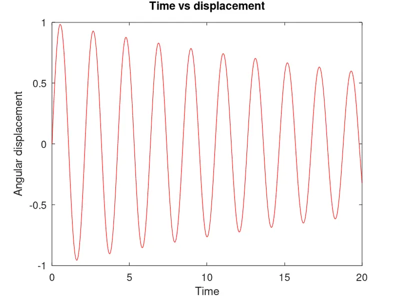
Plot for angular displacement vs time is as follows

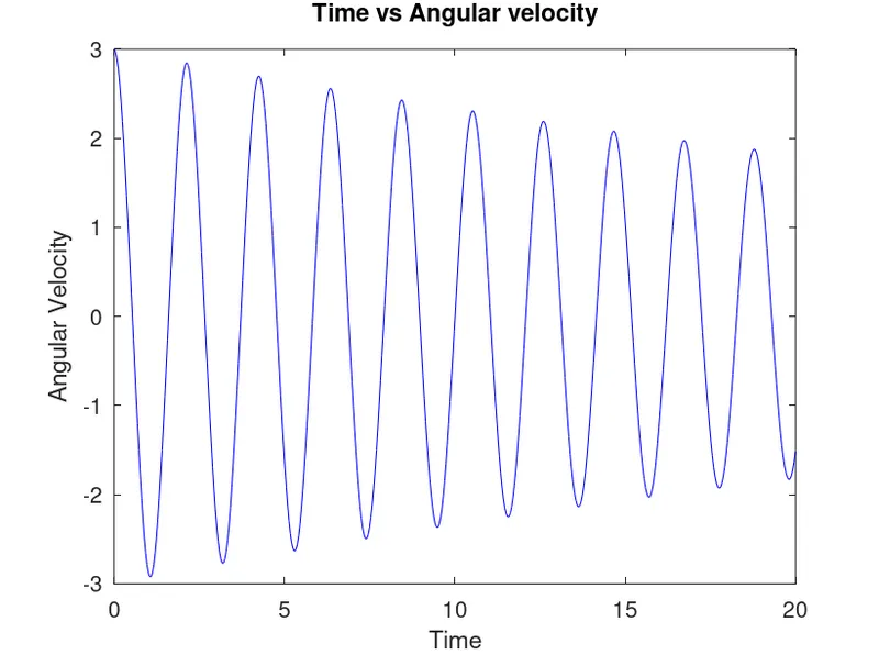
Plot for angular velocity vs time

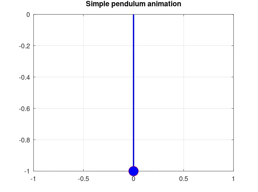
Animation of a simple pendulum with damping

RESULT:

• In the above program displacement vs time for pendulum was calculated by solving second order differential equation and the plot for same shows how displacement is affected for a time span and how it slows down due to effect from mass gravity and friction /damping effect from the air.
• Also, Angular velocity vs Time also shows how it is affected for movement through the mean position of the pendulum as it is highest at that point while zero for reaching its boundary position at the two ends, and that range decreases with time by natural constraints for damping and gravity

CONCLUSION:

Second-order differential equation solving by ode45 command gives us a brief idea of how we should divide an equation of second-order differential equation into 2 first-order differential equations. Likewise, various applications of second-order differential equations can be solved and practical use of Matlab can be seen and achieved.