Week 4.1 - Genetic Algorithm

AIM: To optimize the stalagmite function and find the global maxima of the function.

INTRODUCTION:

The stalagmite function is a mathematical equation that returns a function to define an upward-growing mound of mineral deposits that have precipitated from water dripping onto the floor of a cave. Its Mathematical representation is followed as below

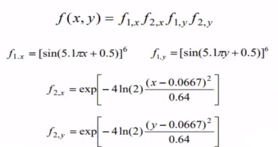
Where x,y are the input variables.

Program for simple stalagmite representation

clear all
close all
clc

%Range of input varaiables
x=linspace(0,0.6,150);
y=linspace(0,0.6,150);

%calling the stalagmite function and calculate the x,y varaible inputs.
for i=1:length(x)
    for j=1:length(y)
        inp(1)=x(i);
        inp(2)=y(j);
        f(i,j)=stalagmite(inp);
    end
end
%plot of stalagmite in 3d
figure(1)
hold on
surfc(x,y,-f)
xlabel('X axis')
ylabel('Y axis')
shading interp

Stalagmite Function:

function [f]=stalagmite(inp)
%input variable subdivied into 2 x,y
  x=inp(1);
  y=inp(2);
  %functions
  f1=(sin((5.1*pi.*x)+0.5)).^6;
  f2=(sin((5.1*pi.*y)+0.5)).^6;
  f3=exp((-4*log(2)).*((x-0.667).^2)/0.64);
  f4=exp((-4*log(2)).*((y-0.667).^2)/0.64);
  f5=(f1.*f2.*f3.*f4);
  %-ve sign to get the following from down to up
  f=-f5;
end

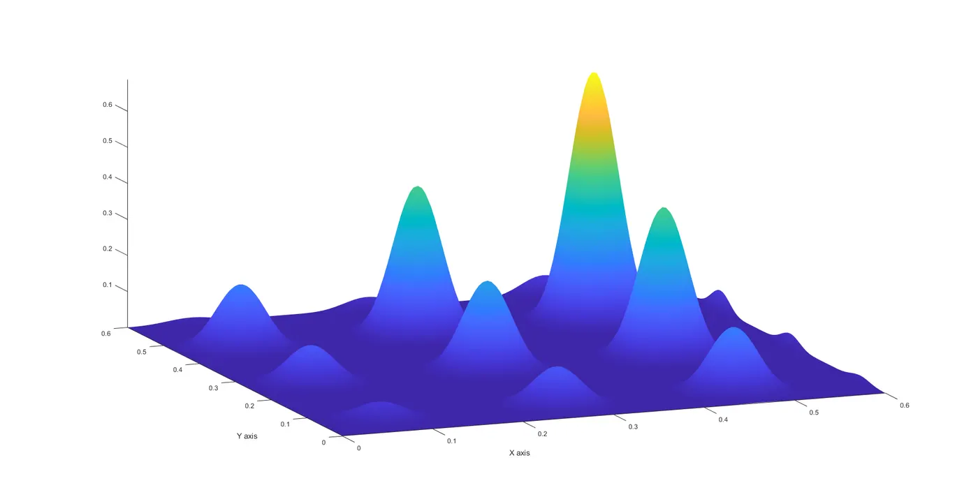
Plot for Simple Stalagmite:

GENETIC ALGORITHM:

Based on the science of evolution by natural selection by Sir Charles Darwin, this algorithm is commonly used for solutions to optimization and search problems by the method of selection, mutation, and crossover. It revolves around the theory of natural selection of the fittest candidates from a population and they create offspring which inherit the characteristics of their parents. There are 5 phases for the genetic algorithm:-

• Initial population
• Fitness Function
• Selection
• Crossover
• Mutation

Initial Population:

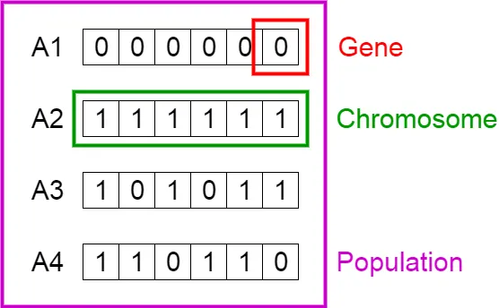
The range of values is selected in which each value is a solution. Each value is Set of Genes called chromosomes.

2. Fitness Function:

It Defines how close a value is to an optimal solution of a function, the higher the fitness value closer it is to be an optimal solution of a problem. The fitness function in this problem is the stalagmite function.

3. Selection:

Based on the fitness function those who satisfy the criteria are selected.

4. Crossover:

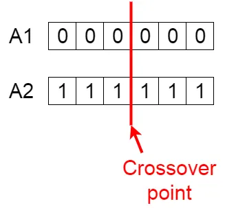
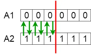
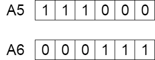
Pair of parents are selected and randomly a crossover point is generated and by exchanging genes up till that point an offspring is created. The new offspring is then added to the population. The below figure shows the same.

5. Mutation:

In Mutation an offspring's random gene value is inverted.

Termination of Algorithm happens when no new offspring is generated then the collection of those last generated offspring is considered as the best solution to a problem.

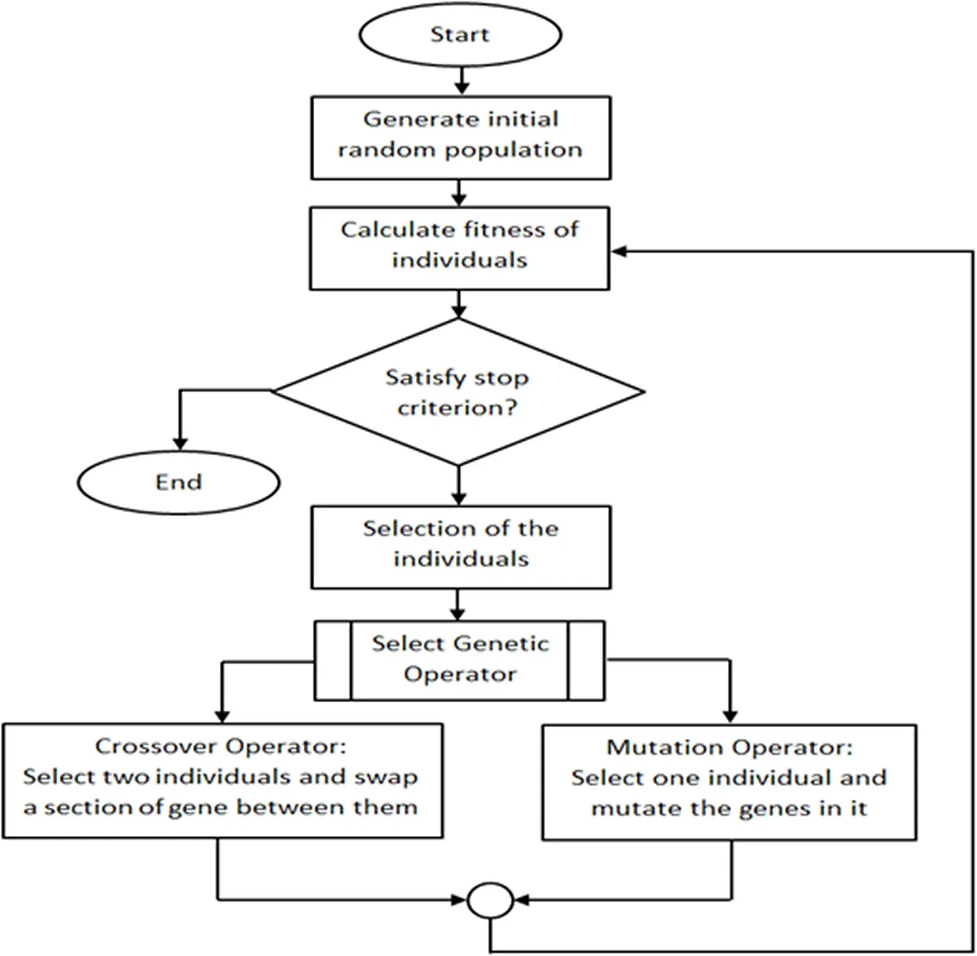
Flowchart :

GENETIC ALGORITHM in MatLab

A function called ga is available to get an optimal solution.

The syntax for ga function are as below:

[x,fval]=ga(fun,nvars)

[x,fval]=ga(fun,nvars,A,b,Aeq,beq)

[x,fval]=ga(fun,nvars,A,b,Aeq,beq,lb,ub)

[x,fval]=ga(fun,nvars,A,b,Aeq,beq,lb,ub,nonlcon)

[x,fval]=ga(fun,nvars,A,b,Aeq,beq,lb,ub,nonlcon,IntCon,options)

Program for optimization and solution to Stalagmite using Genetic algorithm.

function [f]=stalagmite(inp)
%input variable subdivied into 2 x,y
  x=inp(1);
  y=inp(2);
  %functions
  f1=(sin((5.1*pi.*x)+0.5)).^6;
  f2=(sin((5.1*pi.*y)+0.5)).^6;
  f3=exp((-4*log(2)).*((x-0.667).^2)/0.64);
  f4=exp((-4*log(2)).*((y-0.667).^2)/0.64);
  f5=(f1.*f2.*f3.*f4);
  %-ve sign to get the following from down to up
  f=-f5;
end
​

clear all
close all
clc


%Range of input varaiables
x=linspace(0,0.6,150);
y=linspace(0,0.6,150);
%no of iterations
numxl=100;

%calling the stalagmite function and calculate the x,y varaible inputs.
for i=1:length(x)
    for j=1:length(y)
        inp(1)=x(i);
        inp(2)=y(j);
        f(i,j)=stalagmite(inp);
    end
end
  
  

%case Study 1: Unbounded conditions

tic %timer start command
for i=1:numxl
  [inl,fila(i)]=ga(@stalagmite,2);
  xopt(i)=inl(1);
  yopt(i)=inl(2);
end
study1_time=toc %timer end command
figure(1)
subplot(2,1,1)
hold on
%Surface plot to display Stalagmite
surfc(x,y,-f)
xlabel('xx')
ylabel('yy')
%to remove line on surface plot
shading interp
%solutions and function value to plot for unbounded region
plot3(xopt,yopt,-fila,'marker','o','markersize',5,'markerfacecolor','r')
colorbar
title('unbounded inputs')
subplot(2,1,2)
%iterations vs function values
plot(-fila,'linewidth',1,'color','r')
xlabel('iterations')
ylabel('Function maximum')


%case Study 1: Bounded conditions

tic  %timer start command
for i=1:numxl
    [in2,fila2(i)]=ga(@stalagmite,2,[],[],[],[],[0;0],[0.6;0.6]);
      xopt1(i)=in2(1);
      yopt1(i)=in2(2);
end
study2_time=toc   %timer end command
figure(2)
subplot(2,1,1)
hold on
%Surface plot to display Stalagmite
surfc(x,y,-f)
xlabel('xx')
ylabel('yy')
%to remove line on surface plot
shading interp
%solutions and function value to plot for unbounded region
plot3(xopt1,yopt1,-fila2,'marker','o','markersize',5,'markerfacecolor','r')
colorbar
title('bounded inputs')
subplot(2,1,2)
%iterations vs function values
plot(-fila2,'linewidth',1,'color','r')
xlabel('iterations')
ylabel('Function maximum')

%case Study 3: Bounded Condition with optimal options selected

tic   %timer start command
options=optimoptions('ga','populationsize',4000)
for i=1:numxl
    [in4,fila4(i)]=ga(@stalagmite,2,[],[],[],[],[0;0],[0.6;0.6],[],[],options);
      xopt2(i)=in4(1);
      yopt2(i)=in4(2);
end
study3_time=toc  %timer end command
figure(3)
subplot(2,1,1)
hold on
%Surface plot to display Stalagmite
surfc(x,y,-f)
xlabel('xx')
ylabel('yy')
%to remove line on surface plot
shading interp
%solutions and function value to plot for unbounded region
plot3(xopt2,yopt2,-fila4,'marker','o','markersize',5,'markerfacecolor','r')
colorbar
title('bounded inputs')
subplot(2,1,2)
%iterations vs function values
plot(-fila4,'linewidth',1,'color','r')
xlabel('iterations')
ylabel('Function maximum')

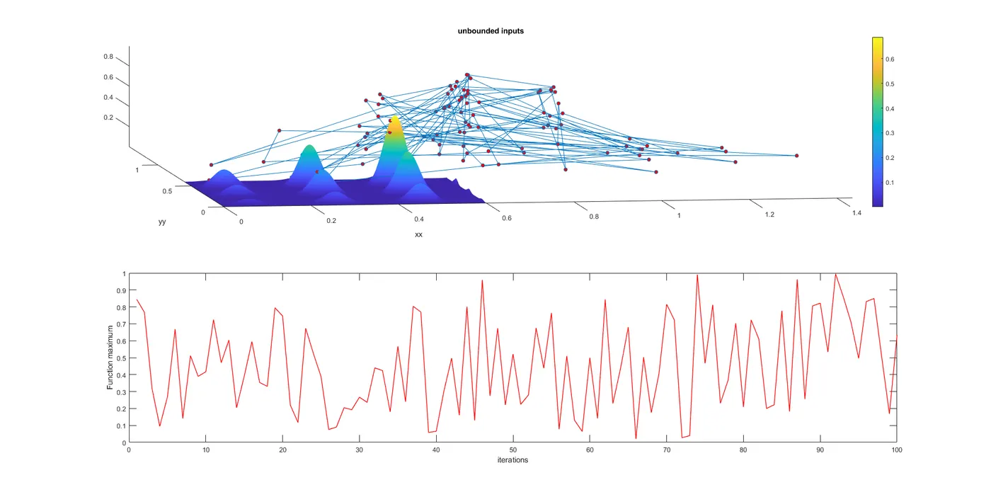
• Here there were no bounds for running the ga code it automatically sampled a population for our function and calculated a set of solutions for the stalagmite function and it is all over the place.
• So this is not an optimal solution.

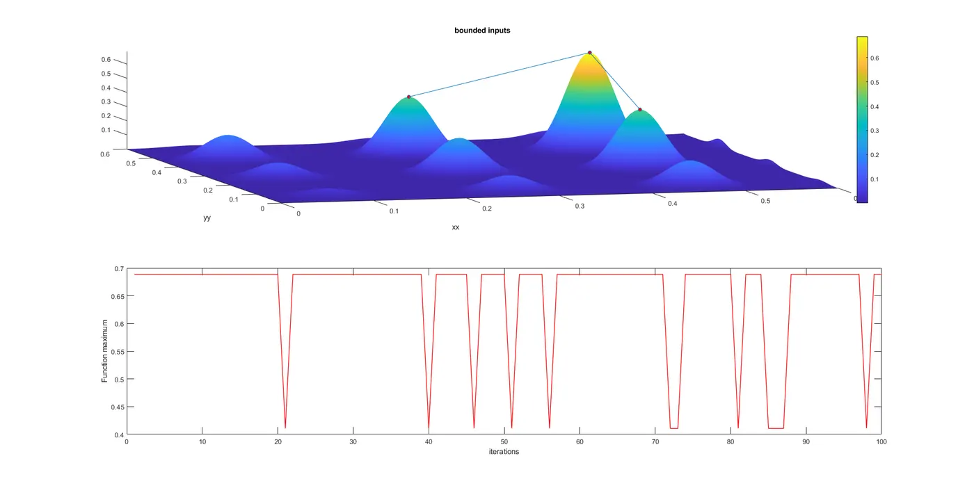
• Bounded the function for the range of 0 to 0.6 in both parameters and let it select population from this range,
• It gives three solutions to our global maxima for stalagmite.

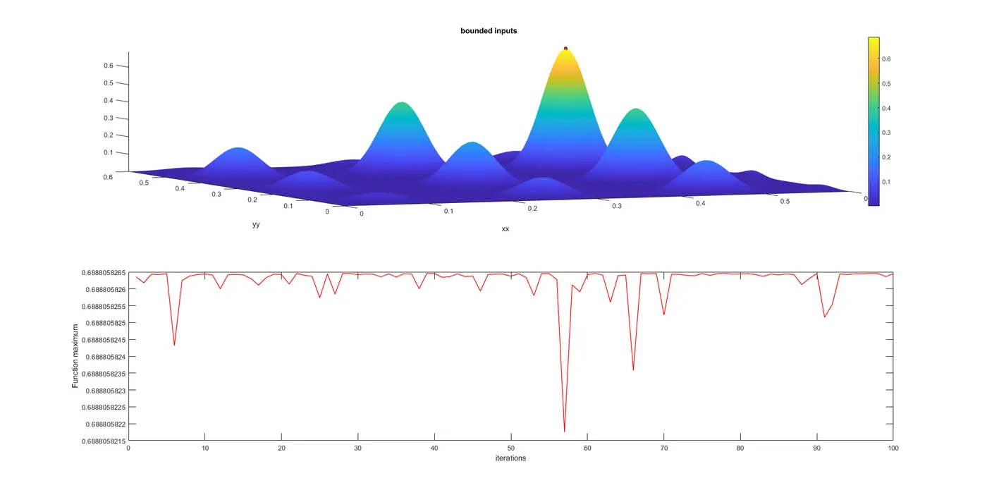
• Selecting bound with a select population size of 4000 gives the only global maxima for our stalagmite function problem.

• Induced the global maxima for stalagmite function using genetic algorithm with optimal.
• Found solutions for all 3 cases of unbound, bounded & bounded with optimoptions command in ga.
• Plotted graphs and surface plots for 3 studies and for F maximum vs no. of iterations.

• Genetic algorithm helps in generating optimal solution to a given function problem and it reduces a lot of time in problem-solving compared to the brute-Force method of function solving.

• Introduction to Genetic algorithm
• Syntax for GA code