Rankine cycle Simulator Using MATLAB

AIM:

• Create a Rankine Cycle Simulator using OCTAVE/MATLAB.
• To plot the corresponding T-s and h-s plots.
• Calculate the state points of the Rankine Cycle.

THEORY:

Rankine cycle is a theoretical cycle on which a steam turbine operates to produce work output to generate Electricity. There are 4 major processes in a Rankine cycle namely, Isentropic Expansion, Constant pressure heat, Isentropic Compression, Constant pressure heat addition by the boiler. Below is a diagram of a simple Rankine cycle

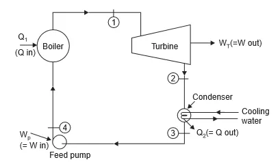
Figure: 1

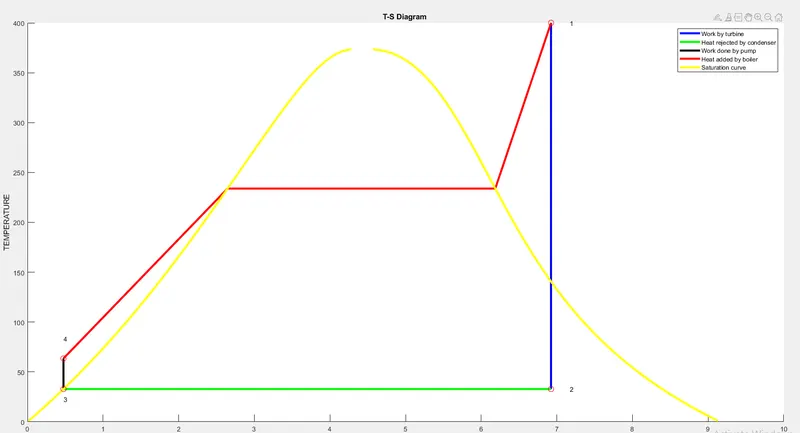
Here Heat is provided in the boiler to heat water and change the phase from liquid to gas and increase pressure. this superheated/heated steam is delivered to the turbine which produces work output. Then the low-pressure low-temperature steam is supplied to the condenser where it changes phase from gas to liquid at the same pressure. The feed pump then pumps the water from the condenser back into the boiler and hence cycle keeps ongoing. The T-S diagram of the Rankine cycle is as follows:

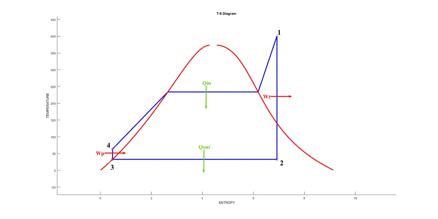
Figure: 2

In the above figure

• 1-2 is Isentropic Expansion in the Turbine
• 2-3 is Constant pressure heat rejection in the Turbine
• 3-4 is Isentropic Compression in the Pump
• 4-1 is Constant pressure heat addition by the boiler

Calculations to be done on Rankine cycle

Considering the mass of fluid as 1kg

Steady Flow energy Equation:

where Q = Heat transfer rate. (J/s)

W = Work transfer rate. (J/s)

△h = Difference in Enthalpy(J/kg)

Applying steady flow energy equation (S.F.E.E.) to boiler, turbine, condenser, and pump :

Boiler state 1:

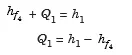
here, hf4 = Enthalpy of fluid at the pump.

h1 = Enthaply of fluid after the boiler.

Q1 = Heat transfer rate by the boiler to the fluid.

Turbine state 2:

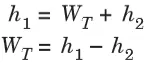
here, Wt = Work done by the turbine.

h2 = Enthalpy of fluid after the turbine.

Condenser state 3:

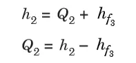
here, Q2 = Heat transfer rate by condenser from fluid to surrounding.

hf3 = Enthalpy of fluid after the condenser.

Pump state 4:

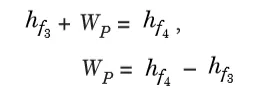
here, Wp = Work done by the pump.

The efficiency of the Rankine cycle.

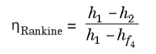
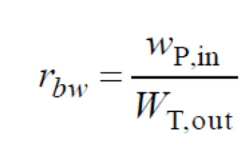
Back work ratio :

Dryness fraction:

In figure 2 we can see that the entropy of state 1 and 2 are equal despite the temperature range so by acquiring the value of h1 and s1 from the steam table for given temperature and pressure. By comparing the equations dryness fraction can be calculated as follows.

MATLAB PROGRAM

To calculate efficiency and work ratio of Rankine cycle for the given input

• Turbine Inlet temperature = 400° C
• Turbine Inlet Pressure = 30 bars
• Turbine Outlet Pressure = 0.05 bars = Condenser Inlet Pressure

clear all
close all
clc
fprintf('                         RANKINE CYCLE SIMULATORn')

%input from user for p1,p2,t1
p1=input('ENTER THE INLET TURBINE PRESSURE P1 in bar=');
p2=input('ENTER THE INLET TURBINE TEMPERATURE P2 in bar=');
t1=input('ENTER THE OUTLET TURBINE PRESSURE T1 in C=');
%STATE 1 finding h1 and s1 from steam table function
h1=XSteam('h_pt',p1,t1);
s1=XSteam('s_pt',p1,t1);

%STATE 2 finding hf,sf,hg and sg from steam table function and determing
%dryness fraction for h2
s2=s1;
hf=XSteam('hL_p',p2);
sf=XSteam('sL_p',p2);
sg=XSteam('sV_P',p2);
hg=XSteam('hV_P',p2);
x=(s2-sf)/(sg-sf);
h2=hf+(x*(hg-hf));
t2=XSteam('Tsat_p',p2);



%STATE 3 h3 and s3 already found while calculating dryness fraction
h3=hf;
s3=sf;
t3=t2;
p3=p2;


%STATE 4 finding h4 and s4 b y finding pump0 work
p4=p1;
v3=XSteam('vL_p',p2);
Wp=v3*(p1-p2);
h4=Wp+h3;
s5=XSteam('sL_p',p1);
s4=s3;
t4=h4/(s5-s4);


%HEAT ADDED , HEAT REJECTED and TURBINE WORK
Qin=h1-h4;
Qout=h2-h3;
Wt=h1-h2;

%To find saturation point for pressure 1 to plot in T-S diagram 
t5=XSteam('Tsat_p',p1);
t6=t5;
s6=XSteam('sV_p',p1);
N=1-(Qout/Qin);
Wr=(Wp)/Wt;

%Printing of all values at each states
fprintf('ntttt1-2  is Isentropic  Expansion  in the Turbinentttt')
fprintf('2-3  is Constant pressure heat rejection  in the Turbinentttt')
fprintf('3-4  is Isentropic  Compression  in the Pumpntttt')
fprintf('4-1  is Constant pressure heat addition by the boiler')
fprintf('nnntttttttRESULTSn==========================================================================================n ')
fprintf('STATE 1ttttSTATE 2tttttSTATE 3tttt STATE 4')
fprintf('nP1=%f barttP2=%f bartttP3=%f bartt P4=%f barn',p1,p2,p3,p4)
fprintf('T1=%f CtttT2=%f CtttT3=%f Ctt T4=%f C',t1,t2,t3,t4)
fprintf('nH1=%f kJ/kgtH2=%f kJ/kgtH3=%f kJ/kgt H4=%f kJ/kg',h1,h2,h3,h4)
fprintf('nS1=%f kJ/kgKttS2=%f kJ/kgKttS3=%f kJ/kgKt S4=%f kJ/kgK',s1,s2,s3,s4)
fprintf('nttttttx=%fnEFFICIENCY=%f  nBACK WORK RATIO = %fn',x,N*100,Wr)
fprintf('Heat added by boiler = Qin = %f kJ/Kgn',Qin)
fprintf('Heat removed by condenser = Qout = %f kJ/Kgn',Qout)
fprintf('Work Output by Turbine = Wt =%f kJ/Kgn',Wt)
fprintf('Work done by pump = Wp =%f kJ/Kgn',Wp)

%To find saturation points for plotting the saturation curves
T=linspace(1,375,500);
for i=1:length(T)
    sf(i)=XSteam('sL_T',T(i));
    sg(i)=XSteam('sV_T',T(i));
    hf(i)=XSteam('hL_T',T(i));
    hg(i)=XSteam('hV_T',T(i));
end


%PLOT of TS with saturation curve
figure(1)
hold on 
plot([s1 s2],[t1 t2],'linewidth',3,'color','b')
plot([s2 s3],[t2 t3],'linewidth',3,'color','g')
plot([s3 s4],[t3 t4],'linewidth',3,'color','k')
plot([s4 s5 s6 s1],[t4 t5 t6 t1],'linewidth',3,'color','r')
plot(sf,T,'color','y','linewidth',3)
plot(sg,T,'color','y','linewidth',3)
plot(s1,t1,'marker','o','MarkerSize',8,'MarkerEdgeColor','red')
plot(s2,t2,'marker','o','MarkerSize',8,'MarkerEdgeColor','red')
plot(s3,t3,'marker','o','MarkerSize',8,'MarkerEdgeColor','red')
plot(s4,t4,'marker','o','MarkerSize',8,'MarkerEdgeColor','red')
text(s1+0.25,t1,'1')
text(s2+0.25,t2,'2')
text(s3,t3-10,'3')
text(s4,t4+20,'4')
xlabel('ENTROPY')
ylabel('TEMPERATURE')
title('T-S Diagram ')
legend('Work by turbine','Heat rejected by condenser','Work done by pump','Heat added by boiler','Saturation curve')

%PLOT of H-S with saturation curve
figure(2)
hold on

plot([s1 s2],[h1 h2],'linewidth',2,'color','b')
plot([s2 s3],[h2 h3],'linewidth',2,'color','g')
plot([s3 s4],[h3 h4],'linewidth',2,'color','k')
plot([s4 s1],[h4 h1],'linewidth',2,'color','cyan')
plot(sf,hf,'color','r','linewidth',2)
plot(sg,hg,'color','r','linewidth',2)
xlabel('ENTROPY')
text(s1,h1,'1')
text(s2,h2,'2')
text(s3,h3,'3')
text(s4,h4+120,'4')
ylabel('ENTHALPY')
title('H-S Diagram ')
legend('Work by turbine','Heat rejected by condenser','Work done by pump','Heat added by boiler','Saturation Curve')

OUTPUT

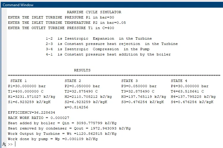
Command Window

PLOTS:

1. T-S Diagram

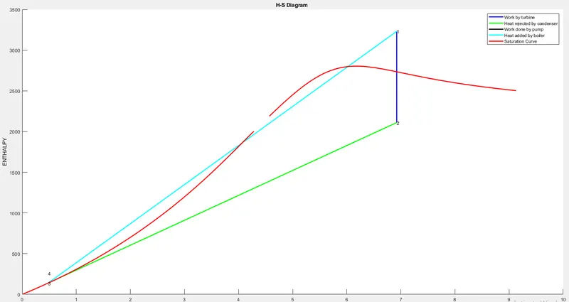
2.H-S Diagram

RESULTS:

• The efficiency for the Rankine cycle in the above example is 36.22%
• The back work ratio is 0.000027
• Plotted H-S and T-S diagram with saturation curve.

REFERENCES:

1. R. K. Rajput - Engineering Thermodynamics_ A Computer Approach (SI Units Version), Third Edition-Jones & Bartlett Publishers (2009)