Solving second order ODEs using MATLAB

Week 3 - Solving second order ODEs using MATLAB

AIM:

(1) Write logic to solve the second-order differential equation for a simple pendulum motion.

(2) Use the marker command to create working animation video for a simple pendulum motion.

BRIEF:

The pendulum is a body or mass suspended from a fixed point so that it can swing back and forth under the influence of gravity. The periods depends on the pendulum and also to a slight degree on the amplitude, the width of the pendulum's swing.

To find the displacement and velocity for the given system, we derivate the second-order differential equation into 2 variables to solve in the MATLAB solver using ode45:

`(d^2theta)/dt^2 + (b/m) (d theta)/dt + (g/l) sin theta = 0`

Considering,

`theta =theta_1`

`(d theta)/dt = (d theta_1)/dt = theta_2`

`(d^2theta)/dt^2 = (d^2 theta_2)/dt^2 = d/dt((d theta_1)/dt) = d/dt (theta_2)`

`therefore (d^2 theta_1)/dt^2 + (b/m) (d theta_1)/dt + (g/l) sin theta_1 = 0`

`(d theta_2)/dt + (b/m) theta_2+ (g/l) sin theta_1 = 0`

We got two variables for the above equation:

`(d theta_1)/dt = theta_2`

`(d theta_2)/dt = -(b/m) theta_2 - (g/l)sin theta_1`

INPUTS PARAMETERS:

(1) Length of the pendulum, `l=1 m`

(2) Mass of the bob, `m=1 kg`

(3) Damping coefficient, `b=0.05`

(4) Gravitational accleration,` g = 9.81m/s^2`

CODE LOGIC:

(1) Firstly, we define the input variables as per mentioned the question such as the length of the pendulum, the mass of the bob, damping coefficient and the constant of gravitational acceleration.

(2) Assigning the value of angular velocity `theta` as per the displacement with respect to time.

(3) Solve the second-order ODEs, using the ode45 function, which is the predefined partial differential equation solver using the numerical method in MATLAB. As the order is 2, we need 2 variable i.e `theta_1` & `theta_2` to solve the problem.

(4) The ode45 function is called out into the mail code by providing the required output and plot the graph showing the curve for 'Displacement vs Velocity' for the given value of `theta` for the particular time span.

Syntax : [t, results] = ode45(@(t,theta) ode_func(t,theta,b,g,l,m),t_span,theta_0)

(5) For creating the line diagram of the simple pendulum, we use the marker command to create the support bar, a hinge or pivot, the string of the pendulum and the bob (sphere) by assigning the corresponding values.

(6) For creating the animation of the pendulum, we need to define the values of bob w.r.t. to 'x' & 'y' axis.

At initial, `x_0= 0` & `y_0= 0`

At final, `x_1= lsin(theta)` & `y_1= -lcos(theta)` [negative sign indicated the downward axis of the string]

(7) After that we can use movie command to store this animation into a small AVI clip.

CODE:

(1) The function code:

%Second Order Differential equation function

function [dtheta_dt] = ode_func(t,theta,b,g,l,m)

theta1 = theta(1)
theta2 = theta(2)
dtheta1_dt = theta2;
dtheta2_dt = -(b/m)*theta2-(g/l)*sin(theta1);
dtheta_dt = [dtheta1_dt;dtheta2_dt];
end

(2) Main code:

%Second Order ODEs for Simple Pendulum 

close all     %close all the window
clear all     %clear the workspace window      
clc           %clear the command window 


%Input parameters
b = 0.05;         %damping co efficient
g = 9.81;         %gravitational acceleration
l = 1;            %length of the string
m = 1;            %mass of bob

%initial condition
theta_0 = [0;3];      %Displacement & Velocity

%time points 
t_span = linspace(0,20,500);

%solve ODE
[t, results] = ode45(@(t,theta) ode_func(t,theta,b,g,l,m),t_span,theta_0);

plot (t,results(:,1))
figure (1)
hold on
plot (t,results(:,2))
grid on
ylabel ('Plot')
xlabel ('Time')
legend ('Displacement','Velocity')
title ('Motion of Pendulum')

%Animation
ct = 1;
for i = 1:length(results(:,1))
    x0 = 0;
    y0 = 0;
    x1 = l*sin(results(i,1));
    y1 = -l*cos(results(i,1));
    
    figure (2)
    plot (x0,y0,'-square', 'MarkerSize',10, 'MarkerFaceColor','r','MarkerEdgeColor','r','color','r') 
    hold on
    plot ([x0 x1],[y0 y1],'-','MarkerSize',2, 'MarkerFaceColor','b','MarkerEdgeColor','b','linewidth', 2,'color','b')
    plot (x1,y1,'o', 'MarkerSize',10, 'MarkerFaceColor','r','MarkerEdgeColor','r')
    plot ([-1 1], [0 0], 'linewidth',2, 'color','g')
    grid on
    axis ([-2 2 -2 2])
    pause (0.1)
    M(ct) = getframe(gcf);
    hold off
    ct = ct + 1;
end

movie(M)
videofile = VideoWriter('pendulum_swing_animation.avi','Uncompressed AVI');
open(videofile)
writeVideo(videofile,M)
close(videofile)

ERRORS:

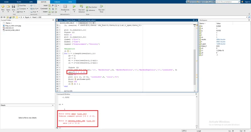
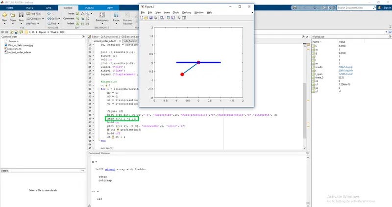
(1) The error in the string of axis. Strings are assigned inside the parenthesis.

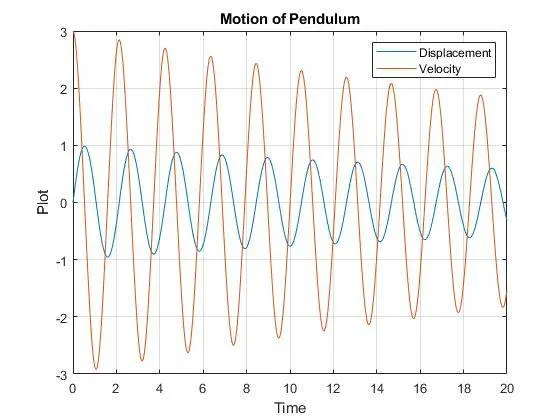
RESULTS: Looking at the graph, we can say that by changing the damping co-efficient we can reduce the displacement and the velocity in the given system.

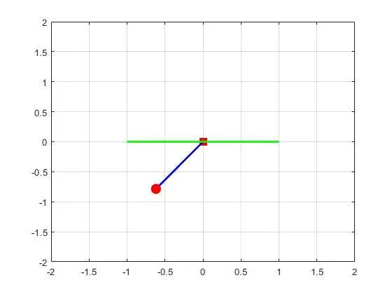
The 2D line diagram of the simple pendulum using the marker's command.

CONCLUSION:

Successfully created a program to solve the second-order ODE to simulate the simple pendulum motion and create a working animation for the same.

Animation video:

https://drive.google.com/file/d/1AOoeugg156Q7GmeE9E6d8xRFKLTukw8w/view?usp=sharing