PYTHON Week 3 - Solving second order ODEs
AIM:
To code using second order differential equation using the formula mention below for simple pendulum.
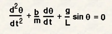
OBJECTIVE
The main objective of this challenge is to code the simple pendulum and simulate using python programming.
1) Plotting the graph for (time vs plot) for displacement and velocity.
2) Animating the simple pendulum by giving appropriate values to the plotting command.
For inputs of specific values in the formula, the details of the pendulum are given:
L= 1
m= 1
b= 0.05
g= 9.81
THEORY
A simple pendulum consisting of a mass hanging from a string of length L and fixed at pivot point P. when displaced to an initial angle and released, the pendulum will swing back and forth with the periodic motion. By applying newtons second law for rotational systems the equation for a motion to be obtained as:
 ,
,
and rearranged as.
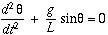 .
.
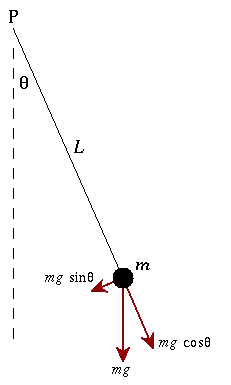
Fig 1: Pendulum
For doing in the python for this challenge the above-mentioned equation to be solved by writing the code.
PROCEDURE:
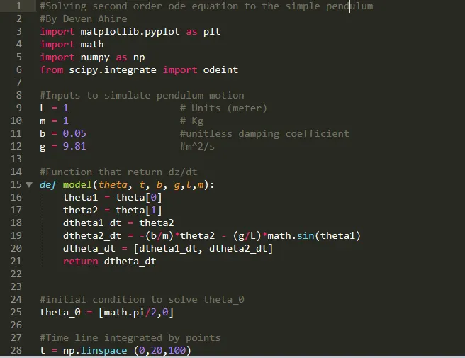
A) Writing code for the animation of the pendulum:
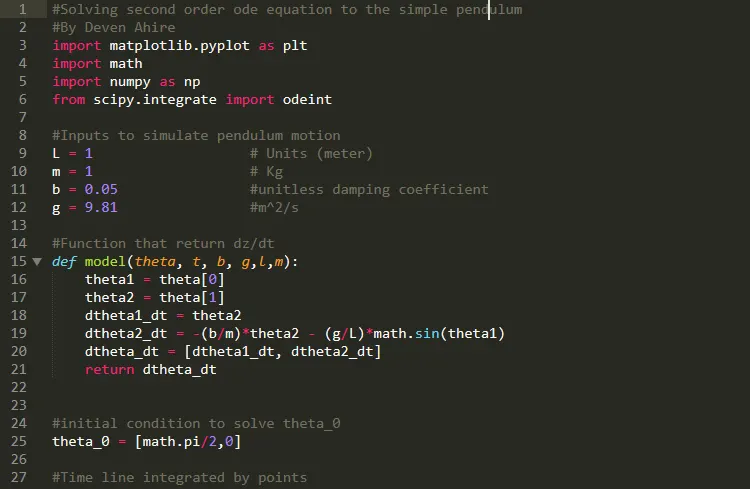
- Importing the scipy and numpy module for integrating the second-order differential equation and for plotting the graph matplotlib and also for the mathematical equation math module.
- # Inputs (L = 1 # Units (meter)
m = 1 # Kg
b = 0.05 #unitless damping coefficient
g = 9.81 #m^2/s) - Defining the value of dθ_1 for that model the (theta, t, b, g,l,m):
theta1 = theta[0]
theta2 = theta[1]
dtheta1_dt = theta2
dtheta2_dt = -(b/m)*theta2 - (g/L)*math.sin(theta1)
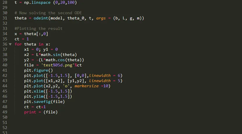
dtheta_dt = [dtheta1_dt, dtheta2_dt] and then return the value to dtheta_dt. - For the time to be divide into the points, the linspace command is used from 0 to 200 by 100 for swing.
- To solve the ode eqution odeint command from scipy is used as mention: theta = odeint(model, theta_0, t, args = (b, L, g, m)).
- To get the figure in x-limit and y-limit and to arrange each figure properly mention below:
- x = theta[:,0]
ct = 1
for theta in x:
x1 = 0; y1 = 0
x2 = L*math.sin(theta)
y2 = -(L*math.cos(theta))
file = 'test%05d.png'%ct
plt.figure()
plt.plot([-1.5,1.5], [0,0],linewidth = 6)
plt.plot([x1,x2], [y1,y2], linewidth = 5)
plt.plot(x2,y2, 'o', markersize =10)
plt.xlim([-1.5,1.5])
plt.ylim([-1.5,1.5])
plt.savefig(file)
ct = ct+1
print = (file)
#Solving second order ode equation to the simple pendulum
#By Deven Ahire
import matplotlib.pyplot as plt
import math
import numpy as np
from scipy.integrate import odeint

#Inputs to simulate pendulum motion
L = 1                   # Units (meter)
m = 1                   # Kg
b = 0.05                #unitless damping coefficient
g = 9.81                #m^2/s

#Function that return dz/dt
def model(theta, t, b, g,l,m):
	theta1 = theta[0]
	theta2 = theta[1]
	dtheta1_dt = theta2
	dtheta2_dt = -(b/m)*theta2 - (g/L)*math.sin(theta1)
	dtheta_dt = [dtheta1_dt, dtheta2_dt]
	return dtheta_dt


#initial condition to solve theta_0
theta_0 = [math.pi/2,0]

#Time line integrated by points
t = np.linspace (0,20,100)

# Now solving the second ODE
theta = odeint(model, theta_0, t, args = (b, L, g, m))

#Plotting the result
x = theta[:,0]
ct = 1
for theta in x:
	x1 = 0; y1 = 0
	x2 = L*math.sin(theta)
	y2 = -(L*math.cos(theta))
	file = 'test%05d.png'%ct
	plt.figure()
	plt.plot([-1.5,1.5], [0,0],linewidth = 6)
	plt.plot([x1,x2], [y1,y2], linewidth = 5)
	plt.plot(x2,y2, 'o', markersize =10)
	plt.xlim([-1.5,1.5])
	plt.ylim([-1.5,1.5])
	plt.savefig(file)
	ct = ct+1
	print = (file)
B) Writing code for the plotting graph for acceleration and velocity:
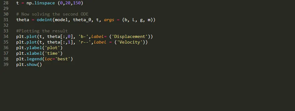
- For this following the same process except instead of plotting command for the figure value, xlabel and ylabel plotted by name them as acceleration and velocity.
- The time vs plot graph has been plotted.
#Solving second order ode equation to the simple pendulum
#By Deven Ahire
import matplotlib.pyplot as plt
import math
import numpy as np
from scipy.integrate import odeint

#Inputs to simulate pendulum motion
L = 1                   # Units (meter)
m = 1                   # Kg
b = 0.05                #unitless damping coefficient
g = 9.81                #m^2/s

#Function that return dz/dt
def model(theta, t, b, g,l,m):
	theta1 = theta[0]
	theta2 = theta[1]
	dtheta1_dt = theta2
	dtheta2_dt = -(b/m)*theta2 - (g/L)*math.sin(theta1)
	dtheta_dt = [dtheta1_dt, dtheta2_dt]
	return dtheta_dt


#initial condition to solve theta_0
theta_0 = [math.pi/2,0]

#Time line integrated by points
t = np.linspace (0,20,150)

# Now solving the second ODE
theta = odeint(model, theta_0, t, args = (b, L, g, m))

#Plotting the result
plt.plot(t, theta[:,0], 'b-',label= ('Displacement'))
plt.plot(t, theta[:,1], 'r--',label = ('Velocity'))
plt.ylabel('plot')
plt.xlabel('time')
plt.legend(loc='best')
plt.show()
RESULT:
The output plotting graph of acceleration and velocity where it states the wavelength of the acceleration start from 1.5 and acceleration starts from 0 as it provided accurate results for the coding. As the result states that angular displacement and angular velocity as it changes over time due to the damping effect and it reduces with respect to the time as shown in the plot.
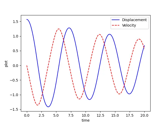
Fig 2: Time Vs plot graph
2) The youtube video link has shared to swing of the pendulum:
APPENDIX:
Coding for the animation of a simple pendulum:
Coding for acceleration and velocity graph:
Error
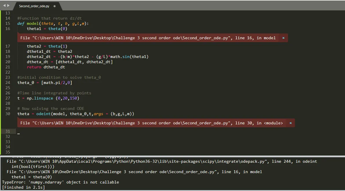
Inline 16 after theta bracket was not given properly because of it the numpy was not callable.
-----------------------------------------------------------------------------------------------------------------------------------------------------------------------------------------------------------------
Model and file link: https://drive.google.com/drive/folders/19GfydreXk1NsStocpkatryY2ZZN_VQAr?usp=sharing