Week 3 - Solving second order ODEs

AIM:

To solve a second order ordinary differential equation (ODE) using the MATLAB.

OBJECTIVE:

To understand how to solve the ODE using MATLAB and to simulate the pendulum motion with the given time.

PROGRAMME:

1). Programme for solving Second order ODE.

clear all
close all
clc

% Inputs
l = 1;
m = 1;
b = 0.05;
g = 9.81;

% Initial conditions
theata_0 = [0;3];

% Time span
t_span = linspace(0,20,500);

% Solve ODE
[t, results] = ode45(@(t,theata) ode_func(t, theata, b,g,l,m),t_span, theata_0);

% Plotting
hold on
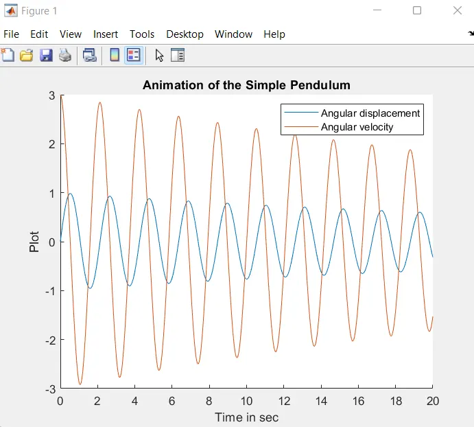
plot(t,results(:,1))
plot(t,results(:,2))
xlabel('Time in sec')
ylabel('Plot') 
title('Damped harmonic motion of the Simple Pendulum')
legend('Angular displacement', 'Angular velocity')

% To create animation of simple Pendulum
ct = 1;
theata_1 = results(:,1);

for i = 1:length(results(:,1))

    % Starting Co-ordinates
    x_start = 0;
    y_start = 0;
    theata_2 = theata_1(i);

    % Ending Co-ordinates
    x_end = 1*sin(theata_2);
    y_end = 1*cos(theata_2);

    % Plotting of Simple Pendulum
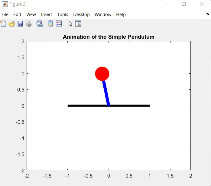
    figure(2)

    % Base of Pendulum
    plot([-1,1],[0,0],'linewidth',4,'color','black')
    hold on

    % String of Pendulum
    line([x_start x_end], [y_start y_end],'linewidth',6,'color','b')
    hold on

    % Bob of Pendulum
    plot(x_end,y_end, 'marker','o','markersize',28,'markerfacecolor','r')
    axis([-2 2 -2 2])
    pause(0.03)
    title('Animation of the Simple Pendulum')
    hold off
    M(ct) = getframe(gcf);
    ct = ct+1;

end
% To create a movie 
movie(M)
videofile = VideoWriter('simple_pendulum.avi','uncompressed AVI');
open(videofile);
writeVideo(videofile,M);
close(videofile);

2). Programme to create a Function.

function [dtheata_dt] = ode_func(t,theata,b,g,l,m)

theata1 = theata(1);
theata2 = theata(2);
dtheata1_dt = theata2;
dtheata2_dt = -(b/m)*theata2 - (g/l)*sin(theata1);
dtheata_dt = [dtheata1_dt; dtheata2_dt];

end

EXPLANATION:

• To solve the ODE of simple pendulum with damping, inputs and variables has been defined, such as Damping coefficient (b), length of the spring (l), mass of the bob (m) and gravity (g).
• Initial conditions such as angular displacement and angular velocity for the given time has been defined, where as the time span is defined by the linspcae command to get a smooth graphical representaion of the values.
• Hence further to solve ODE, ode45 is used which is the inbuilt function in Matlab, whereas (t, theata) is constant and we introduce another fucntion called ode_func in which the second order ode is break down to the two first order ode and input values and variables are assigned to the function, then the result has been calculated with respect to time.
• Plot command is used to plot the solved ode with respect to time.
• To create a animation of simple pendulum for loop is used in which the starting and ending co-ordinates have been calculated, then the base of the pendulum, string of the pendulum and bob of the pendulum are plotted using plot and line commands.
• Animation of the pendulum is created using the Movie command where as each frames are captured and made into a movie.

ATTACHMENTS:

1).

2).

3).

4).

5).

ERRORS OCCURED:

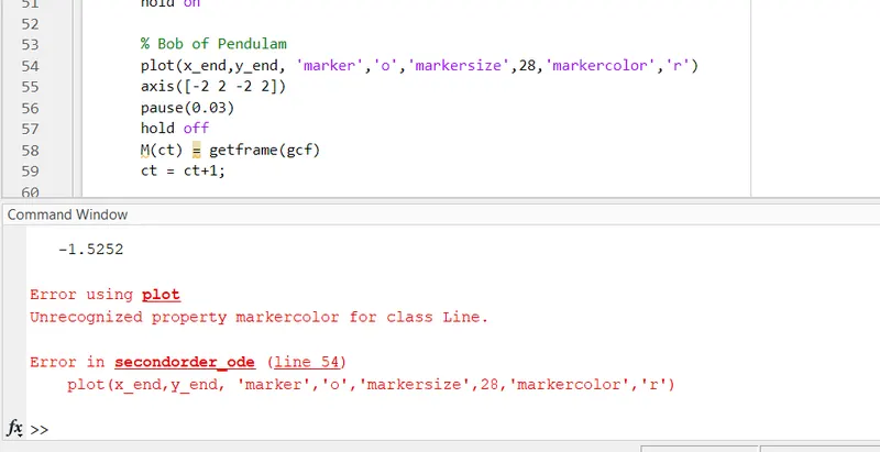
• Error occured in the attachment 4 is that, in the line 54 markerfacecolor has been mistakenly entered as markercolor which leads to unrecognized property error, then it has been rectified
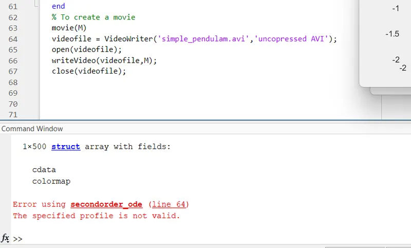
• Error in attachment 5 is that, in line 64 uncompressed AVI has been mistakenly written later rectified.

ANIMATION:

• https://drive.google.com/file/d/1rvMF1eGfqOaEqu_vMQEa40XJS3fKpcKx/view?usp=sharing

RESULT:

From this above programme we understood how to solve the ODE using Matlab, damped harmonic motion of the simple pendulum is usnderstood by the graphical representation and the Animation of the simple pendulum is created.