Week 3 - Solving second order ODEs

pendulum_animation1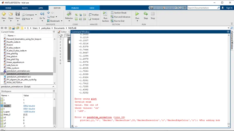

clear all
close all
clc

%Inputs
b = 0.05; %damping coefficients
m = 1; %mass of the bob
g = 9.81; %acceleration due to gravity
l = 1; %length of chord

%Initial Displacement,Initial Velocity
theta_0 = [0,3] %angular diplacement and angular velocity

%Time
t_span = linspace(0,20,500); %generate values from 0 to 20 for 100

%ODE
[t,results] = ode45(@(t,theta)ode_func(t,theta,b,g,l,m),t_span,theta_0)

ct = 1;
for i = 1:length(results(:,1));

    x0 = 0;  %Coordinates for the fixed point of the pendulum
    y0 = 0;

    x1 = l*sin(results(i,1)); %Vertical line for the chord
    y1 = -l*cos(results(i,1)); %Horizontal line of the chord

    %Plotting
    plot([-1 1],[0 0],'linewidth',4,'Color','b'); %Plot for the chord movement
    hold on
    plot([x0 x1],[y0 y1],'linewidth',2,'color','b'); %Chord moving
    hold on
    plot(x1,y1,'v', 'Marker','o','MarkerSize',20,'Markerfacecolor','r','MarkerEdgeColor','r'); %For adding bob
    hold off;
    grid on;
    axis([-1.5 1.5 -1.5 1.5]); %Defining the axis for the graph
    pause(0.03);
    M(ct) = getframe(gcf) %Capturing the frames of the pendulum movement
    ct = ct+1; %incrementing the counter
end

movie(M) %Calling the frames
pendulum_animation1 = VideoWriter(['pendulum_animation1.avi'],'uncompressed avi') %Writing the video
open(pendulum_animation1) %open the video
writeVideo(pendulum_animation1,A) %Perform the frames to video
close(pendulum_animation1) %Close the file


function[dtheta_dt] = ode_func(t,theta,b,g,l,m)

       theta1 = theta(1)
       theta2 = theta(2)
       dtheta1_dt = theta2;
       dtheta2_dt = -(b/m)*theta2 - (g/l)*sin(theta1);
       dtheta_dt = [dtheta1_dt; dtheta2_dt];
end





This program is regarding simulation of the pendulum motion.
Here, basically first priority is about solving the ordinary differential equation, which is done using ODE45 inbuilt solver in MATLAB.
Starting with clearing all the old data. Next, we gave inputs i.e., damping coefficients, mass of the bob, acceleration due to gravity, length of the rod.
Then, we define initial angular displacement and angular velocity. After this we define time range from 0 to 20 using ‘linspace’ command, according to given values.
Then we get result using ODE45 function, to get animation we need to get values on x and y plan.
For that purpose, ‘for’ loop is used where we define loop counter variable, which gives us x1,y1 values.
To plot the graph coordinates are assigned, ‘marker’ command with symbol ‘o’ is used to get sphere shape for the bob.
Then we define axis and to capture the frames of the pendulum movement we use command ‘getframe’.
Then to save video in avi format we use 'VideoWrite' and 'WriteVideo' Commands



ERRORS ENCOUNTERED
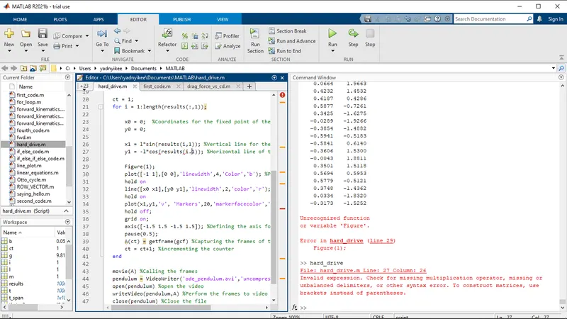
1. In first image, in case of y1 there should have been ‘comma’ but by mistake I used 
   ‘full stop’. This photo shows this error, on this realization I changed it to 
   ‘comma’.
2. In the second image the error is about not using marker symbol i.e., ‘o’. which is 
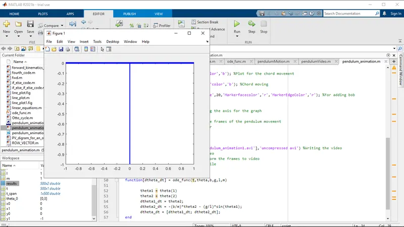
   why I did not get bob in the animation. The kind if output I got is shown in the next 
   photo.
3. As I entered symbol, ’o’, I got proper output
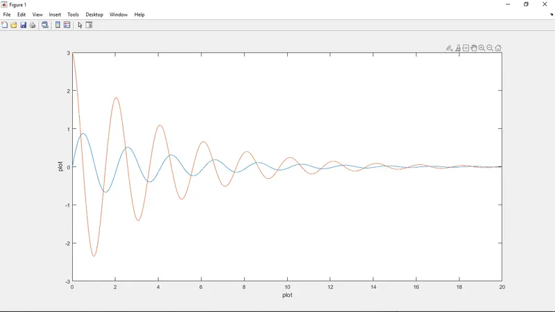
4. Image which shows the curves is the output of the given ODE representing motion of 
   the simple pendulum.


  

pendulum_animation link - https://youtu.be/iTLl3pxL6_o