Project 1
%%%%%%%%%%%%%%%%%%%%%%%%%%%%%%%%%%%%%%%%%%%%%%%%%%%%%%%%%%%%%%%%%%%%%
%% Skill-Lync -> Hybrid Drives Development
% Project 1 - Conventional Vehicle Model
% By - Ullekh Gambhira
% Description:
%% Initialization File
% Initialization file for loading the variables for the Conventional vehicle simulation model
%% Vehicle Parameters
M = 1500; % Vehicle weight [kg]
Cr = 0.015; % Rolling resistance coefficient
Rw = 0.35; % Rolling radius [m]
Cd = 0.33; % Drag coefficient
Af = 2; % Frontal area [m2]
rhoa = 1.225; % Air density [kg/m3]
Vwind = 0; % Wind velocity [kmph]
g = 9.81; % Gravitational acceleration [m/s2]
theta = 0; % Slope [deg]
myu_road_tire = 1; % Coefficient of friction between tire - road interface
%% Powertrain Parameters
FDR = 3.73; % Final Drive Ratio / Diff Ratio
DiffEff = 0.99; % Differential efficiency (assumed independent of operating conditions)
NumGear = 4; % Number of gears in transmission
TransGear = [1:NumGear]; % Transmission Gears
TransRatio = [3.06, 1.62, 1, 0.7]; % Corresponding Transmission ratios
TransEff = 0.90; % Transmission efficiency (assumed independent of operating conditions)
TC_SR = [0, .5, .6, .7, .8, .87, .92, .94, .96, .97, 1]; % Torque Converter Speed Ratio (Matlab default) -> TurbSpd/PumpSpd
TC_TR = [2.232, 1.5462, 1.4058, 1.2746, 1.1528, 1.0732, 1.0192, 1, 1, 1, 1]; % Torque Converter Torque Ratio (Matlab default) -> TurbTrq/PumpTrq
TC_Cf = 1e-4 * [.72558, .66322, .63463, .59042, .51331, .4144, .29287, .22444, .12186, .04386, 0]; % Torque Converter Capacity Factor (Matlab default) -> PumpTrq/PumpSpd^2 [Nm/rpm^2]
load Vehicle_Data/Engine_data_1_9L_Saturn_95kW
load Vehicle_Data/Trans_Shift_map
%% Driver Parameters
Kp = 10; % P gain for driver PI model
Ki = 1; % I gain for driver PI model
Drive_Cycle_Select = 1; % Drive cycle selection
% Drive cycle values in m/s
if Drive_Cycle_Select == 1
load DriveCycles/UDDS;
elseif Drive_Cycle_Select == 2
load DriveCycles/HWFET;
elseif Drive_Cycle_Select == 3
load DriveCycles/FTP;
elseif Drive_Cycle_Select == 4
load DriveCycles/US06;
elseif Drive_Cycle_Select == 5
load DriveCycles/NEDC;
elseif Drive_Cycle_Select == 6
load DriveCycles/WLTP;
end
time_end = cyc_time(end);
vel_end = cyc_vel(end);
%%%%%%%%%%%%%%%%%%%%%%%%%%%%%%%%%%%%%%%%%%%%%%%%%%%%%%%%%%%%%%%%%%%%%
%% Skill-Lync -> Hybrid Drives Development
% Project 1 - Conventional Vehicle Model
% By - Ullekh Gambhira
% Description:
% The following file is to used with the Initialization file and Simulink
% results for post-processing of the data.
% The file is incomplete, has some examples of how the data is imported
% into a readable format, data analysis and plotting examples.
% Based on the project task, use commands in a similar format as given
% below, to analyse the data and generate required plots.
% You can change variable names if desired
%% Post-Processing File
% File for post-processing the Conventional vehicle simulation model data
%% Renaming variables
Time = out.tout;
Acc_Pdl = out.Acc_Pdl; % Accelerator pedal [%]
Brk_Pdl = out.Brk_Pdl; % Brake pedal [%]
Gear_Cmd = out.Gear_Cmd; % Transmission gear
Trans_In_Spd = out.Trans_In_Spd*30/pi; % Transmission input speed [rpm]
Trans_Out_Spd = out.Trans_Out_Spd*30/pi;% Transmission output speed [rpm]
Eng_Trq = out.Eng_Trq; % Engine brake torque [Nm]
Eng_Spd = out.Eng_Spd*30/pi; % Engine speed [rpm]
Eng_Fuel_Consump = out.Eng_Fuel_Consumption; % Engine fuel consumption [g]
Veh_Dist = out.Veh_Dist/1000; % Distance traveled by vehicle [km]
Veh_Spd = out.Veh_Spd*18/5; % Vehicle speed [kmph]
Eng_Fuel_Rate = out.Eng_Fuel_Rate;
%% Data Analysis
Eng_Pwr = Eng_Spd.*pi./30.*Eng_Trq./1000; % Engine brake power [kW]
rho_petrol = 0.7197; % Density of petrol [kg/L]
kmpl = Veh_Dist(end)/(Eng_Fuel_Consump(end)/1000/rho_petrol); % Fuel economy [kmpl]
%% Plotting vehicle characteristics time trace
figure()
subplot(3,1,1)
hold on
grid on
plot(Time, Acc_Pdl, 'linewidth', 1, 'Color', 'black');
plot(Time, Brk_Pdl, 'linewidth', 1, 'Color', 'red');
ylabel('Pedal [%]')
xlim([0, Time(end)]);
legend('Accel','Brake');
subplot(3,1,2)
hold on
grid on
plot(Time, Trans_In_Spd, 'linewidth', 1, 'Color', 'black');
plot(Time, Trans_Out_Spd, 'linewidth', 1, 'Color', 'red');
ylabel('Speed [rpm]')
xlim([0, Time(end)]);
ylim([0, 6000]);
legend('Trans Input','Trans Output');
subplot(3,1,3)
hold on
grid on
plot(Time, Gear_Cmd, 'linewidth', 1, 'Color', 'black');
xlim([0, Time(end)]);
xlabel('Time [s]');
ylabel('Gear');
%% Plotting engine operating points on engine fuel map
figure('Name','Engine Operating Points');
hold on
grid on
title('Engine Operating Points','fontsize',12);
p1=plot(Eng_map_spd*30/pi,Eng_max_trq,'linewidth',2,'color','r');
p2=line([Eng_map_spd(end)*30/pi Eng_map_spd(end)*30/pi],[0 Eng_max_trq(end)]);
set(p2,'linewidth',1,'linestyle','--','color','k');
p3=line([Eng_map_spd(1)*30/pi Eng_map_spd(1)*30/pi],[0 Eng_max_trq(1)]);
set(p3,'linewidth',1,'linestyle','--','color','k');
[c,h] = contour(Eng_map_spd'*30/pi,Eng_map_trq,Eng_fuel_map');
clabel(c,h);
xlabel('Engine Speed [rpm]');
ylabel('Engine Torque [Nm]');
title('Engine Fuel Consumption Map [g/s]');
p4 = plot(Eng_Spd,Eng_Trq);
legend([p1 p4],{'Max Curve','Operating Points'});
axis([Eng_map_spd(1)*30/pi Eng_map_spd(end)*30/pi 0 Eng_map_trq(end)]);
%% Plotting engine torque,engine power,fuel rate and fuel consumption
figure()
subplot(4,1,1)
hold on
grid on
plot (Eng_Trq)
xlabel('Time')
ylabel('Engine Torque')
subplot(4,1,2)
hold on
grid on
plot(Eng_Pwr)
xlabel('Time')
ylabel('Engine power')
subplot(4,1,3)
hold on
grid on
plot(Eng_Fuel_Rate)
xlabel('Time')
ylabel('Fuel rate')
subplot(4,1,4)
hold on
grid on
plot(Eng_Fuel_Consump)
xlabel('Time')
ylabel('Fuel Consumption')
%% Plotting acceleration and break pedal,gear command,vehicle desired and
%%actual speed, vehicle distance
figure()
subplot(4,1,1)
hold on
grid on
plot(Time, Acc_Pdl, 'linewidth', 1, 'Color', 'black');
plot(Time, Brk_Pdl, 'linewidth', 1, 'Color', 'red');
ylabel('Pedal [%]')
xlim([0, Time(end)]);
legend('Accel','Brake');
subplot(4,1,2)
hold on
grid on
plot(Time, Gear_Cmd, 'linewidth', 1, 'Color', 'black');
xlim([0, Time(end)]);
xlabel('Time [s]');
ylabel('Gear');
subplot(4,1,3)
hold on
grid on
plot(Veh_Spd, 'linewidth', 1, 'Color', 'black')
plot(Time, Trans_Out_Spd,'linewidth', 1, 'Color', 'red')
xlabel('Time')
ylabel('Speed')
xlim([0, Time(end)]);
legend('Actual Speed','Desired Speed');
subplot(4,1,4)
hold on
grid on
plot(Veh_Dist)
xlabel('Time')
ylabel('Vehicle Distance')
UDDS
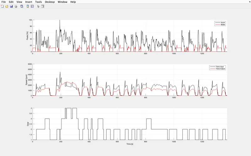
When there is no gear ratio selected or it is at 1, there is no transmission input or output speed and also brakes are applied, It implies vehicle is at rest. When gear ratio is highest transmission output speed is high and acceleration is also highest, it simply means vehicle is at its maximum performance.
As this plot how's the UDDS condition, in urban as we know there is lot of breaking which is shown in the plot. So, keeping in mind we can design vehicle suitable for such condition.
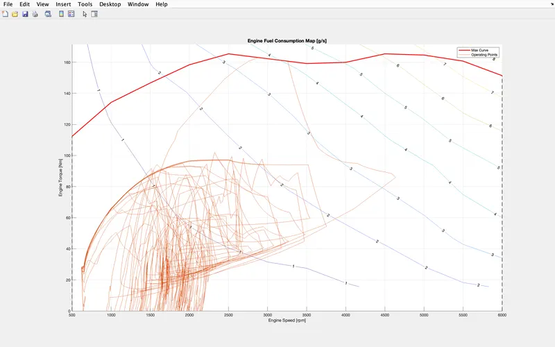
This is the engine fuel consumption map, Here we can see that at Engine Speed 2500 and 4500 torque and engine fuel consumption is highest. Above plot also shows the operating region of the engine which is till 4th gear.
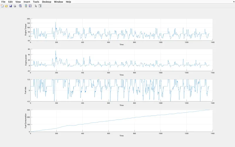
Above plot shows the time trace of engine torque,engine power,fuel rate and fuel consumption, we can also see the variation in Engine torque, Engine Power and Fuel rate respective to each other. We can see here fuel rate is increasing along with the time.
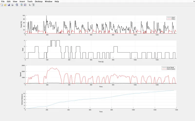
This plot show that there is so much variation in actual speed and desired speed.We can also see along with time vehicle is capturing more and more distance which is very obvious. The difference between the desired speed and actual speed shows the % of losses in the system.
HWFET
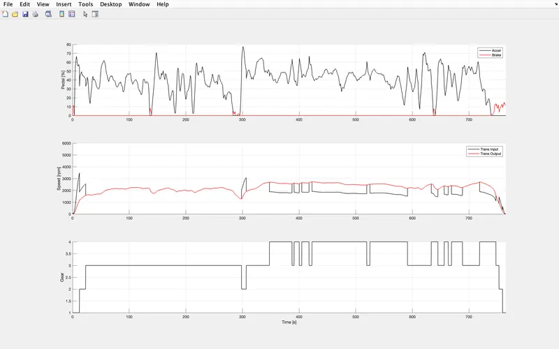
This plot shows the condition of HWFET i.e. highway. Here we can see breaking is very less and acceleration is at high rate. Also we see the transmission output speed is also more compared to input speed. Gear is at its highest ratio for most of the time.
This is engine fuel consumption map. The orange lines shows the operating point.
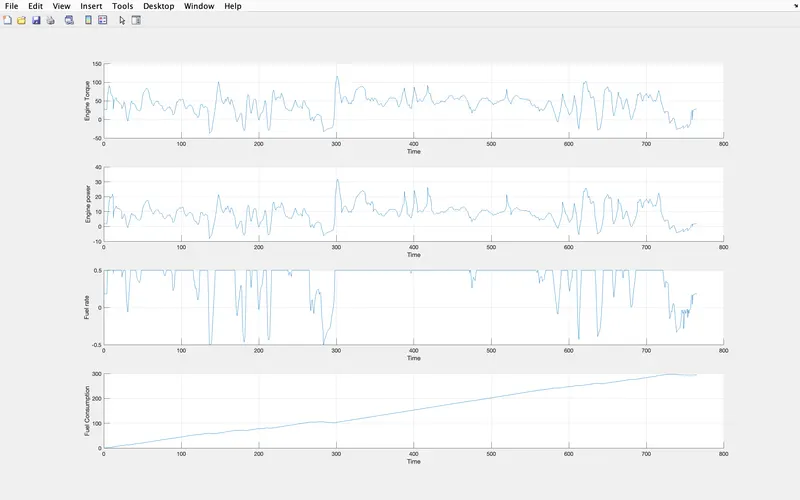
Here we can see time trace of various parameters i.e. engine torque, engine power,fuel rate and fuel consumption. one significant difference as compared to UDDS is that because here we have very less braking fuel rate seems to constant for some amount of time.
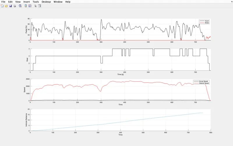
Here we can see there is so much difference between the actual speed and the desired speed.
a] kmpl for UDDS = 28.7791
kmpl for HWFET = 40.2714
This values shows us that fuel economy is high in HWFET as compared to UDDS. As we know on highway there is less traffic compared to urban area which leads to the smoother vehicle travel.
That's why fuel economy rate is more in HWFET.