Week 3 - Solving second order ODEs

Introduction:

The equation given for the problem is generally used to understand the behavior of the pendulum. If we replace displacement(x) instead of angular displacement(theta), it can be used to solve the modal analysis of structures.

By using Matlab, I tried to simulate the motion of the pendulum. This can be achieved by using the given equation to get the position of the body at a given point of time and its angular velocity.

clear
close all
clc

%mass of the ball   m "kg"
%damping coefficient, b "Nm/s"
%length of pendulum, L "m"
%acceleration due to gravity,g "m/s^2"
%Angular displacement of pendulum, theta_d "rad"
%Angular Velocity of pendulum, theta_v "rad/s"
%Initial conditions, initial_conditions [theta_d(0);theta_v(0)]
%time span, t_span "s"
%displacement of pendulem,x "m"
% Movie frames "M"
% Total time "end_time" (s)
% Number of Frames "Frames"


%INPUT

L=1;
m=1;
b=0.05;
g=9.81;
Frames=500;
end_time=20;
t_span=linspace(0,end_time,Frames);
initial_conditions=[0;3];

%SOLUTION

%Solving ode
ode_func=@(t,theta) [theta(2); -(b/m)*theta(2)-(g/L)*sin(theta(1))];
[t,theta]= ode45 (ode_func, t_span, initial_conditions);

%Ploting preparation
theta_d=theta(:,1);
theta_v=theta(:,2);

figure(1)
hold on
plot(t,theta_d)
plot(t,theta_v)
legend("displacement","Velocity")
xlabel("time(s)")
ylabel("angle(rad)")
title("angular displacement and angular velocity with respect to time")
hold off

%Pendulum Movie
fixed_point_x=1.5;
fixed_point_y=1.5;

% Gathering the screenshots
figure(2)

for i =1:length(theta_d)
  clf
  x_inter=fixed_point_x+L*cos(theta_d(i)+deg2rad(270));
  y_inter=fixed_point_y+L*sin(theta_d(i)+deg2rad(270));
  hold on
  plot([fixed_point_x,x_inter],[fixed_point_y,y_inter],"color",[0 0 0],"linewidth", 2)
  plot(x_inter,y_inter,"o","markersize",10)
  axis([0 3 0 2])
  pause(0.01)
  xlabel("Horizontal axis");
  ylabel("Vertical axis");
  title("Motion of the Pendulum");
  M(i)=getframe(gcf);
end
hold off
% Making of Video
figure(3)
movie(M)
videofile= VideoWriter(['pendulum_motion']);
videofile.FrameRate=Frames/end_time;
open(videofile)
writeVideo(videofile,M)
close(videofile)

I solved this equation by using the ode45 solver, for which we are converting a second-order equation into two first-order equations.

Derivation,

Assuming

`theta= theta_1`

`(d^2theta)/dt=(d theta_1)/dt=theta_2`

Then the equation becomes,

`(d theta_1)/dt=theta_2` and

`(d theta_2)/dt=-[(b/m)*theta_2+(g/L)*sin(theta_1)]`

The inputs of the ODE45 are function, time span which contains individual time and the initial condition which is required for solving any ODE equation.

The function which is used for ODE45 must have the above two equations in the form of a matrix and must have time and angular displacement as outputs.

The “@” symbol denotes that function is having two inputs that are dynamically fed to the system.

With the help of the ODE solver, we will get the angular displacement and angular velocity for the pendulum and we can plot the same against time.

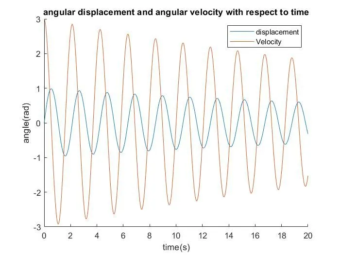
By using trigonometric functions, we can locate the x and y position of the ball.

We can save individual frames by using the getFrame(gcf) function and by using videofile and videoWriter. We can create an animation of the plot.

For setting the video time, we must calculate the required framerate per second(fps) of the video. This can be calculated using the formula below.

`Fps=(Number of Frames)/(Total time)`.

In this way, we can set the time of the video

Video Link: https://youtu.be/OEj3LxgYGeQ